Downscaling Seasonal Precipitation Forecasts over East Africa with Deep Convolutional Neural Networks

Temesgen Gebremariam ASFAW and Jing-Jia LUO

1Institute for Climate and Application Research (ICAR)/CIC-FEMD/KLME/ILCEC,Nanjing University of Information Science and Technology, Nanjing 210044, China

2Institute of Geophysics Space Science and Astronomy, Addis Ababa University, Addis Ababa 1176, Ethiopia

ABSTRACT This study assesses the suitability of convolutional neural networks (CNNs) for downscaling precipitation over East Africa in the context of seasonal forecasting.To achieve this,we design a set of experiments that compare different CNN configurations and deployed the best-performing architecture to downscale one-month lead seasonal forecasts of June–July–August–September (JJAS) precipitation from the Nanjing University of Information Science and Technology Climate Forecast System version 1.0 (NUIST-CFS1.0) for 1982–2020.We also perform hyper-parameter optimization and introduce predictors over a larger area to include information about the main large-scale circulations that drive precipitation over the East Africa region,which improves the downscaling results.Finally,we validate the raw model and downscaled forecasts in terms of both deterministic and probabilistic verification metrics,as well as their ability to reproduce the observed precipitation extreme and spell indicator indices.The results show that the CNN-based downscaling consistently improves the raw model forecasts,with lower bias and more accurate representations of the observed mean and extreme precipitation spatial patterns.Besides,CNN-based downscaling yields a much more accurate forecast of extreme and spell indicators and reduces the significant relative biases exhibited by the raw model predictions.Moreover,our results show that CNN-based downscaling yields better skill scores than the raw model forecasts over most portions of East Africa.The results demonstrate the potential usefulness of CNN in downscaling seasonal precipitation predictions over East Africa,particularly in providing improved forecast products which are essential for end users.

Key words: East Africa,seasonal precipitation forecasting,downscaling,deep learning,convolutional neural networks(CNNs)

1.Introduction

Many potential applications of seasonal climate prediction,including agricultural decision-making,crop yield prediction,and tropical disease prediction,require seasonal climate inputs at much finer spatial resolutions compared with current general circulation models (GCMs;e.g.,Harrison et al.,2007;Meza et al.,2008;Hansen et al.,2011;Ordoñez et al.,2022).Furthermore,due to their coarse spatial resolution,GCMs have limitations in reproducing realistic regional climate features required for the applications mentioned above (e.g.,Doblas-Reyes and Goodess,2005;Gutowski et al.,2020).To date,various statistical and dynamical downscaling methods have been developed to bridge the gap between the coarse-scale information provided by GCMs and the local information required by end-users (e.g.,Tang et al.,2016;Manzanas et al.,2018a;Vandal et al.,2019;Bedia et al.,2020).

As one commonly used approach,dynamical downscaling is based on high-resolution Regional Climate Models(RCMs),driven by boundary conditions from coarse-resolution GCMs.Dynamical downscaling is particularly useful for better simulating convective and extreme precipitation events due to its improved resolution and finer-scale physics representations (e.g.,Giorgi and Gutowski,2015;Sun and Lan,2021),which are often underestimated in statistical downscaling (e.g.,Bürger et al.,2012).However,this method is limited by a lack of intensive computational resources,possible errors from the RCMs,and sensitivity to boundary conditions (e.g.,Vandal et al.,2019;Wang et al.,2021).

As another commonly used approach,statistical downscaling methods establish a statistical relationship between coarse-scale atmospheric variables and high-resolution local observations,and those statistical relationships are subsequently applied to the coarse-scale data to obtain the local variables over a different period or location.Statistical downscaling has an advantage over its dynamical counterpart in terms of computational efficiency while producing equally robust results in simulating the present climate as dynamical models (e.g.,Tang et al.,2016;Vaittinada Ayar et al.,2016;Sun and Lan,2021).Depending on the nature of the predictors chosen during the model calibration,statistical downscaling approaches can be classified either as model output statistics(MOS) or perfect prognosis (PP) approaches (see Maraun et al.,2010 for a review).In MOS,the calibration links predictors from a model to observed predictands,the calibrated model is then used to post-process model output (Maraun and Widmann,2018).In contrast,the PP downscaling approach uses observational data for both predictors and predictands in the training stage and then uses the climate model’s forecast data as predictors in the downscaling stage(e.g.,Gutiérrez et al.,2013;Tian et al.,2014;Manzanas et al.,2018b).The large-scale observations are often replaced by reanalysis products,which assimilate available day-by-day observations into the model space (e.g.,Wilby et al.,2004).

Several previous studies have compared dynamical and statistical downscaling for seasonal precipitation forecasts in different regions of the world (e.g.,Díez et al.,2005;Gutmann et al.,2012;Robertson et al.,2012;Yoon et al.,2012).For instance,Díez et al.(2005) found that both dynamical and statistical (standard analog technique) downscaling methods improve seasonal precipitation forecasts in Spain,but their comparative results from the two methods during the four seasons in Spain are not conclusive.They also reported that,in some of their case studies,the use of dynamical and statistical downscaling methods in combination provides better skill scores than using one of the two methods as an alternative.Yoon et al.(2012) also assessed the potential of a dynamical and two statistical downscaling methods (BCSD and Bayesian) to improve seasonal forecasts in the United States.They found that dynamical downscaling adds values in seasonal prediction applications,that depend on location,forecast lead time,and skill metrics used.Furthermore,they suggested that applying statistical bias correction to the dynamical downscaling outputs improves seasonal forecast skills.

Assessment of the potential improvement using downscaling global forecasts over East Africa is also presented in a few studies (Diro et al.,2012;Buontempo and Hewitt,2018;Nikulin et al.,2018;Tucker et al.,2018;Mori et al.,2021).According to Nikulin et al.(2018) and Tucker et al.(2018),there is no clear improvement offered by dynamical downscaling in terms of seasonal forecast skills.Diro et al.(2012) concluded that the added values using dynamical downscaling in Ethiopia depend on the type of observational data and evaluation metrics used.Their results suggested that the Regional Climate Model (RCM) can improve the probabilistic skill of the global model forecasts,but only when using rain gauges for validation.However,their deterministic assessment showed the RCM’s inability to improve seasonal forecast skills.Diro et al.(2012) and Mori et al.(2021) further reported that dynamical downscaling also causes a sizable systematic error in the precipitation over some parts of East Africa and significantly underestimates the number of wet days during the start of the season.Kipkogei et al.(2017) suggested that their statistically downscaled forecasts demonstrated positive long-term skill in estimating seasonal rainfall amounts,similar to or better than the raw GCM forecasts.Furthermore,based on one case study of precipitation in October-November-December 2015 they found that,although downscaling tends to overestimate rainfall in some parts of the region,it adds realistic spatial details relative to the raw GCM output.

During the past few decades,various statistical downscaling methods have been developed.These methods range from standard statistical methods,such as analogs (Lorenz,1969),generalized linear models (Nelder and Wedderburn,1972),and weather typing (Hewitson and Crane,1996),to more recent and sophisticated machine-learning methods such as artificial neural networks (Wilby et al.,1998),support vector machines (Tripathi et al.,2006),random forests (He et al.,2016;Pour et al.,2016),super-resolution deep residual networks (Wang et al.,2021),and so on.

Recent studies demonstrated that convolutional neural networks (CNN) have a similar or better performance than the classical statistical downscaling methods in downscaling precipitation (e.g.,Pan et al.,2019;Baño-Medina et al.,2020;Sha et al.,2020;Weyn et al.,2020;Wang et al.,2021;Hess and Boers,2022;Vaughan et al.,2022).CNNs also have the ability to extract the most relevant features,which is a difficult task to accomplish in the standard statistical downscaling approaches (e.g.,Baño-Medina et al.,2020,2021).Nevertheless,CNN-based downscaling has not yet been conducted in East Africa;

Therefore,this study employs a CNN model,for the first time for East Africa,to examine its potential in downscaling the seasonal forecasts of June–July–August–September(JJAS) precipitation from the Nanjing University of Information Science and Technology Climate Forecast System version 1.0 (NUIST-CFS1.0).NUIST-CFS1.0 demonstrated exemplary performance in predicting seasonal precipitation and reproducing large-scale dynamics over East Africa(Asfaw and Luo,2022).The study also evaluates the potential added value of CNN-based downscaling in terms of adding spatial details,correcting systematic biases,and improving prediction skills (e.g.,Di Luca et al.,2015;Rockel,2015;Nikulin et al.,2018) of NUIST-CFS1.0 seasonal forecasts of JJAS precipitation over East Africa.

The results and findings of the present study can be applied to support operational seasonal forecasting over East Africa in providing high-resolution local-scale seasonal climate forecasts that satisfy the requirements of impact modelers and farm-level decision-makers.The remainder of this paper is organized as follows.Section 2 provides the data and methods used in this study and section 3 presents the results.Finally,the summary and discussion are given in section 4.

2.Data and methods

2.1.Downscaling domain

The domain of interest for this work is the East Africa region (Fig.1a).To assess the effect of including large area predictors over the downscaling results,we consider two predictor areas (see subsection 2.4.1 for the details): predictors over only the downscaling target region and predictors over a large area (Fig.1b).This large area is particularly suitable to take account of the large-scale meteorological features that drive the East African JJAS season,including the intertropical convergence zone (ITCZ;Nicholson,2017;Seregina et al.,2019,2021),formation of thermal low over North Africa,strengthening of the St.Helena and Mascarene highs,formation and frequency of upper-level and lowerlevel jet features,and cross-equatorial flows (Camberlin,1997;Korecha and Barnston,2007;Nicholson,2017),and the nearby oceans which are the primary moisture sources during the JJAS season (Camberlin,1997;Riddle and Cook,2008;Viste and Sorteberg,2013a,b;Nicholson,2017).

Fig.1.(a) Map of the study area,with elevation (m) and (b) JJAS composite of two typical large-scale predictors,namely the 850-hPa wind (m s–1,vectors) and geopotential height (m,shaded),based on wet years.

2.2.Data

In this study,daily predictors listed in Table 1 from the fifth-generation European Centre for Medium-Range Weather Forecasts (ECMWF) reanalysis (ERA5;Hersbach et al.,2020) were used as predictors to build CNN models in the training phase.Then,the constructed CNN models were applied to the corresponding predictors from each of the nine ensemble members of the NUIST-CFS1.0 forecasts in the prediction phase to obtain the downscaled predictions of seasonal precipitation.This idea was inspired by the PP method,which was introduced in section 1.

Table 1.Predictor variables used in this study.

ERA5 assimilates observations across the globe with an atmospheric model to provide a complete and consistent dataset from 1940 to the present with a 0.25° × 0.25° horizontal resolution and an hourly temporal resolution.The ERA5 data were retrieved from the Copernicus Climate Change Service (C3S;https://cds.climate.copernicus.eu/) for 1981–2020 and were re-gridded to the NUIST-CFS1.0 grid using the nearest neighbor interpolation.

For downscaling,we use predictors from the nine ensemble members of NUIST-CFS1.0 1-month lead forecasts for JJAS,during 1982–2020.Daily gridded rainfall observations from the Climate Hazards Group InfraRed Precipitation with Station (CHIRPSv2;Funk et al.,2015),at a 0.25° resolution,were used as predictand to train the CNN models and as validation reference data.

We implement the two-sample Kolmogorov–Smirnov(KS) test to estimate the distributional similarity between large-scale variables from the ERA5 reanalysis and NUISTCFS1.0 forecasts (not shown here) for the predictors’ selection (e.g.,Gutiérrez et al.,2013;Manzanas et al.,2018b;Baño-Medina et al.,2021).To harmonize the ERA5 reanalysis and the NUIST-CFS1.0 forecast data that are used respectively in the training and prediction phases of the PP approach,NUIST-CFS1.0 monthly mean forecasts are adjusted towards the corresponding climatological reanalysis values as in Maraun (2012) and Bruyère et al.(2014).

2.3.Cross-validation scheme and evaluation metrics

To avoid artificial skill (e.g.,Maraun et al.,2015;San-Martín et al.,2017;Gutiérrez et al.,2019),a five-fold crossvalidation approach was applied.First,the CNN models were trained using four of these blocks and then used to predict the remaining block.In this approach,the period(1981–2020) was divided into five non-overlapping blocks,each containing 32 years for training and 7 or 8 years(1982–88,1989–96,1997–2004,2005–12,and 2013–20)for prediction.The five downscaled series were then stitched into a single series for validation during 1982–2020.

We considered several deterministic and probabilistic evaluation metrics to assess and compare the skills of the raw NUIST-CFS1.0 and the corresponding CNN-based downscaled seasonal predictions of JJAS precipitation.The evaluation metrics are the same as those employed in the recent NUIST-CFS1.0 skill assessment study (Asfaw and Luo,2022).

In addition to JJAS seasonal mean precipitation,we also evaluated the performance of the raw/downscaled daily precipitation forecasts to reproduce the observed precipitation extreme and spell indicator indices,which are of particular interest for many practical applications.Three widely used indices,including the simple daily intensity index (SDII),the relative frequency of wet days (R01),and the 98-th percentile of daily precipitation (P98Wet),are considered(Table 2,see also Maraun et al.,2015;Nikulin et al.,2018;Gutiérrez et al.,2019;Vaughan et al.,2022).These indices have been computed based on daily precipitation time series of the raw and downscaled forecasts and expressed as relative differences with respect to the observed values.

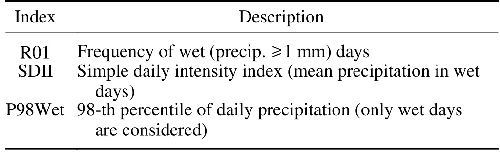
Table 2.Daily precipitation indices used in this study.

2.4.Convolutional Neural Networks (CNNs)

The CNN architecture is based on the CNN model (e.g.,Baño-Medina et al.,2020,2021),which has shown good performance in downscaling daily precipitation over Europe.Based on a series of experiments,we modify the architecture by adding maximum pooling layers,following each convolutional layer,and a dropout layer.We make further changes to the model hyper-parameters by tuning the number of filters in the convolutional layers,kernel size of the convolutional layers,dropout rate,and the number of hidden units in dense layers (see subsection 2.4.1 for details).

Finally,we deploy a CNN-model architecture,which consists of three convolutional layers with 3 × 3 kernels of 32,24,and 16 filter maps,each followed by max-pooling (MP)layers,a dropout layer,two fully-connected (dense) layers with 98 neurons each,and three output layers which estimate the mixed binomial–log-normal distribution parameters of the precipitation model (see Fig.2 for the schematic illustration).

Fig.2.Sketch of the CNN architecture used in this study.The network consists of one input layer (the predictor),three convolutional layers with 3 × 3 kernels of 32,24,and 16 filter maps,each followed by max-pooling (MP)layers,a dropout layer,two fully connected (dense) layers with 98 neurons each,and three output layers which estimate the mixed binomial–log-normal distribution parameters of the precipitation model.The variables of the input layer correspond to 16 coarse (about 1.1°) large-scale standard predictors (see Table 1) in the area of 30°W–90°E and 40°S–40°N.East African (CHIRPS 0.25° × 0.25° grid) precipitation is used as a variable for the output layer.For a more detailed explanation of a similar sketch,please refer to Baño-Medina et al.(2020).

2.4.1.CNN configuration experiments and hyperparameter optimization

The CNN configuration experiment compares existing CNN model configurations and tests the effect of the predictor’s extent,the training season,and the final two layers that link the last hidden layer with the output layers,including additional max pooling and dropout layers.The CNN configurations were trained during 1982–2010,and their forecast performance was validated and compared during the evaluation period of 2011–20 based on the observational datasets.Following the approach proposed by previous downscaling studies (e.g.,Cannon,2008;Baño-Medina et al.,2020,2021;Vaughan et al.,2022),all CNN models in this study are trained to optimize the negative log-likelihood of a Bernoulli-Gamma distribution.The rainfall on a given day is then inferred from a gamma distribution's shape and scale parameters.

The first set of experiments considered the CNN configurations from recent studies on applications of CNN in downscaling climate change projections (e.g.,Baño-Medina et al.,2020,2021) and improving weather prediction (e.g.,Weyn et al.,2020;Hess and Boers,2022).

The CNN configurations considered in this experiment are:

(1) CNN: The CNN configurations are based on the best-performing topologies developed in recent studies on applications of CNN in downscaling climate change projections (Baño-Medina et al.,2020,2021).Furthermore,the CNN model has been reported to outperform the standard statistical downscaling models from the VALUE intercomparison experiments (Gutiérrez et al.,2019).

(2) UNET: U-Net-based CNN (Hess and Boers,2022).This is a modified version of the original U-Net (Ronnebergeret al.,2015;Weyn et al.,2020).Hess and Boers (2022)reported the architecture’s success in improving the forecast skill of relative rainfall frequencies and heavy rainfall events.

Results from the first set of configurations were compared using bias and ACC,and a robust result was found for the CNN.After choosing the CNN over the U-Net,we next attempt to improve the CNN model performance via a screening procedure by varying the extent of the predictors,the training season (JJAS vs the entire 12 calendar months),and the final two layers that link the last hidden layer with the output layers,including the additional max pooling and dropout layers.

(1) CNN-12-month: training the CNN model using the entire 12-month dataset instead of the dataset from the JJAS(June–September) season.

(2) CNN-Transpose: replacing the two dense layers that follow the first block of convolutional layers with transposed convolution layers (Zeiler et al.,2010;Dumoulin and Visin,2018) to increase (up-sample) the spatial dimensions of intermediate feature maps into the output spatial dimensions.

(3) CNN-LA: selecting predictors over a large area (the entirety of Africa,including the nearby oceans) instead of merely over the study area.This large area is particularly suitable to account for the large-scale drivers and primary moisture sources of the precipitation during the East African JJAS season.

(4) CNN-Max pool: applying max pooling (Riesenhuber and Poggio,1999),following each convolutional layer,to reduce the dimensions of the feature maps by a factor of two in both horizontal coordinates while preserving the most important information.Applying pooling layers reduces the number of learnable features in the network and prevent overfitting problems.Among the various types of pooling methods,max pooling is applied here as it selects the maximum element from each pooling window (2×2 in our case),and by doing so it maintains the majority of the dominant features of the feature map while discarding less relevant information (e.g.,Pan et al.,2019;Alzubaidi et al.,2021;Cong and Zhou,2023).

(5) CNN-Dropout: applying dropout,which is suggested by Srivastava et al.(2014) to significantly reduce overfitting and give major improvements over other regularization methods.

After comparing the configurations above,we select the best-performing architecture and further apply hyperparameter tuning to optimize the number of filters in the convolutional layers,kernel size of the convolutional layers,dropout rate,and the number of hidden units in dense layers via the random search optimization strategy (Bergstra and Bengio,2012).Table 3 presents the search space of those model parameters and their optimal values.

Table 3.Search space and optimal values of the model hyper-parameters obtained using optimization.

2.4.2.Scalability experiments

Scalability experiments are used to evaluate the performance of the proposed CNN model in downscaling precipitation using high-resolution predictors from the newer generation of seasonal forecasting systems and reanalysis data sets,which have a typical resolution of 0.25º.The experiments are performed inperfect conditions(e.g.,Maraun et al.,2019;Legasa et al.,2023),using predictors from ERA5 for both training and predicting.Furthermore,1981–2010 and 2011–20 are used as training and validation period,respectively.

ERA5 large-scale variables at their original resolution(0.25º) are used to represent downscaling using fine-resolution predictors,and the corresponding variables are re-gridded to a NUIST-CFS1.0 grid (about 1.1º) to obtain the coarse-resolution predictors.While the observed CHIRPS precipitation is available at 0.05º and 0.25º horizontal resolutions,for consistency,the 0.05º version is upscaled to 0.1º(fine resolution) and 0.25º (coarse resolution) using the bilinear interpolation method.The resultant precipitation at 0.1º(around 12 km) and 0.25º (around 28 km) resolutions are then used as the predictand to train the CNN model using the fine-resolution and coarse-resolution predictors,respectively.

The CNN-based downscaled precipitation amounts at the two spatial scales are compared based on the bias and an anomaly correlation coefficient (ACC) after the precipitation at fine resolution (0.1º) is upscaled to coarse resolution(0.25º) using bilinear interpolation.Downscaling using fineresolution predictors achieves similar bias and a slightly better ACC than that of using coarse-resolution predictors (Fig.S1 in the electronic supplementary materials,ESM),which indicates that the proposed CNN model can be applied to downscale forecasts at higher resolutions.

3.Results

3.1.Comparison of CNN configurations

Comparisons of the aforementioned CNN models’ forecast skills are shown in Fig.3.The boxplots represent the spread of the biases and ACC along the entire observation grid (the blue lines inside the box indicate the median value,whereas the boxes outline the lower and upper quartiles).In general,the biases from the neural networks are smaller(slightly underestimated) than the raw forecasts,except for one of the CNN models that is trained with the whole 12-month dataset (instead of the JJAS seasonal dataset).While using the whole 12-month dataset was expected to increase the model's performance by providing more samples for training–which is usually needed by neural networks–in practice,it caused the model to perform worse than the other CNN models (underestimating the precipitation).This was likely attributed to the dry climatology during the other seasons than JJAS in East Africa.It appears that the increased samples from the dry seasons do not well represent the relations between the predictors and precipitation in the rainy season (i.e.,JJAS) and thus degrade the performance of the CNN model.

Fig.3.Comparison of the CNN models’ forecasts with the raw NUIST-CFS1.0 forecasts.(a) Bias and (b) anomaly correlation coefficients (ACC) between the CNN model’s ensemble mean precipitation and observation during the test period of 2011–20.The box plots represent the spread of the precipitation forecasts over the observed grid (the blue lines inside the box indicate the median value,whereas the boxes outline the lower and upper quartiles).

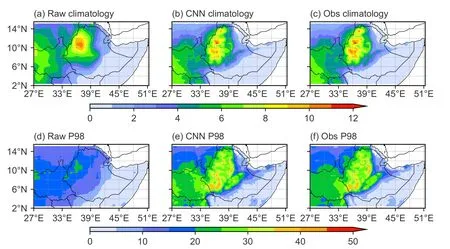
Fig.4.(top panels) JJAS seasonal mean climatology of precipitation (mm d–1) and (bottom panels) the 98-th percentile (P98;mm d–1) during 1982–2020.Left panels: the 9-member ensemble mean of raw NUIST-CFS1.0 forecast initiated from 1 May.Middle panel: downscaled results from the CNN model,and right panel: CHIRPS observational precipitation used for the verification.

In addition,despite adding complexity to the CNN model,which may benefit from learning from complex spatial features,the U-net does not outperform the base CNN as the U-net overfits quickly due to the limited data to train its complex topology.Replacing the two dense layers that follow the first block of convolutional layers with transposed convolution layers reduces the bias.However,it yields lower ACC,suggesting that adding the two dense layers increases the nonlinearity of the model,which better represents the relationship between the predictors and the predictand.

Our results suggest that the CNN model that was trained using large-area predictors (see Fig.1b) delivers better results with low biases and high ACC skills.This indicates that including large-area predictor information helps the CNN to represent the large-scale meteorological features that drive local precipitation and enable the model to perform better at predicting the precipitation anomalies,as indicated by the higher ACC skills.Furthermore,the forecasts were further improved by adding maximum pooling and dropout layers.This suggests that down-sampling the spatial features learned with the convolution layers and dropping 35% of training parameters does not result in a relevant loss of spatial information affecting the downscaling.In contrast,it helps the neural networks to learn more robust features (with emphasis on important features) and reduce overfitting.As a result,the CNN model with maximum pooling and dropout layer provides the highest ACC skills,being overall the best model in predicting the interannual variations of the JJAS precipitation in East Africa.

3.2.Deterministic forecast skill

Figure 4 shows the mean and 98-th percentile (P98)JJAS seasonal precipitation climatology.The left panel corresponds to the raw NUIST-CFS1.0 outputs,the middle panel displays the downscaled results using the best CNN model,and the right panel shows the observations.The raw NUISTCFS1.0 forecast exhibits moderate to large biases of both the mean and P98 precipitation over most parts of East Africa,with a tendency to overestimate precipitation over wet regions of central Ethiopian highlands and underestimate precipitation over dry regions of East Africa.In particular,the NUIST-CFS1.0 forecast highly underestimates the P98 over the central and northern highlands of Ethiopia and South Sudan.In contrast,the CNN-downscaled results better capture the fine spatial distributions of the precipitation over East Africa,particularly the observed precipitation maximums over the western and northern highlands of Ethiopia,and the dry conditions over northeastern Ethiopia and Sudan.This may be due to the CNNs’ ability to extract the relevant spatial features that determine the local precipitation and to model the nonlinear relationship between large-scale meteorological features and local precipitation (e.g.,Baño-Medina et al.,2021).The improvement is much more noticeable for the extreme precipitation (P98),which is particularly important for impact estimations or when computing climate indices depending on absolute values/thresholds (e.g.,Katz and Brown,1992;Manzanas et al.,2019;Vaughan et al.,2022).

The associated biases of the raw and downscaled JJAS mean and P98 precipitation are presented in Fig.5.The CNN model effectively reduces the raw NUIST-CFS1.0 forecast biases,leading to mean errors smaller than 1 mm d–1.Moreover,CNN-based downscaling effectively reduces the widely-extended P98 dry bias in the raw NUIST-CFS1.0 forecasts over the central highlands,western Ethiopia,and South Sudan and even produces slightly overestimated P98 values there.The CNN's significant bias reduction in the mean and P98 climatology is to be expected as it was trained directly with observations (Baño-medina et al.,2022).

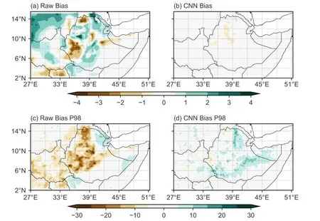
Fig.5.Panels (a) and (b) show the bias (mm d–1) of the JJAS seasonal mean climatology of precipitation,while (c) and (d) show the bias for the P98 (mm d–1) during 1982–2020.The results are based on the 9-member ensemble mean forecasts of the raw NUIST-CFS1.0 (left panels) and the CNN model (right panels).

The deterministic forecast skills of the raw NUISTCFS1.0 and CNN downscaled outputs for the seasonal forecasts of JJAS precipitation during 1982–2020 over East Africa are assessed using the root-mean-square error(RMSE) and ACC (Fig.6).CNN downscaling reduces the large errors in the raw model forecasts over Sudan,the eastern part of South Sudan,and northwestern and southeastern Ethiopia.Moreover,improvement is observed in capturing the interannual variations of precipitation,measured using ACC (Figs.6c,d).The improvement is particularly apparent in South Sudan,Sudan,Eretria,and the northeastern and northern parts of Ethiopia.

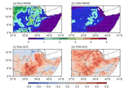
Fig.6.Panels (a) and (b) show the root-mean-square error (RMSE;mm d–1) of the JJAS seasonal mean climatology of precipitation,while (c) and (d) show the anomaly correlation coefficient (ACC) of JJAS seasonal mean rainfall anomalies during 1982–2020,based on the ensemble mean forecast from NUISTCFS1.0 (left panels) and the CNN model (right panels).

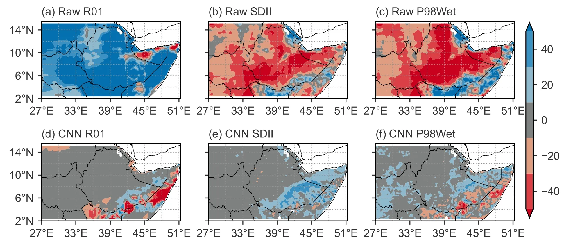
Fig.7.Relative biases of precipitation indices (%) based on (upper panels) the raw NUIST-CFS1.0 and (bottom panels)CNN-based downscaled seasonal forecasts of JJAS precipitation during 1982–2020.The relative biases are computed relative to the CHIRPS observations.

Figure 7 shows the biases of the precipitation extremes and spell indicators obtained from the raw NUIST-CFS1.0 and CNN downscaled forecasts.The results are expressed as a percentage relative to the CHIRPS observed values.We can see that the raw NUIST-CFS1.0 forecast has a large positive relative bias of R01 over the study area.Moreover,it has large negative relative biases for SDII and P98Wet,except over the coast of Somalia and northeast Ethiopia.The underestimated R01 and overestimated SDII and P98Wet are due to the drizzling problem in most current GCMs (e.g.,Dai,2006;Sun et al.,2006;Chen and Dai,2019),within which the simulated precipitation has the correct amount but falls as a drizzle over many days instead of in distinct heavy precipitation events.

On the other hand,the CNN downscaled predictions show a clear improvement in predicting the extreme and spell indicators,which yield substantially lower biases.Remarkably,CNN-based downscaling corrected the raw model's positive bias of R01 and the negative bias of SDII and P98Wet over most parts of East Africa.However,the CNN slightly underestimates R01 and inherits the positive bias of SDII and P98Wet exhibited by the raw NUISTCFS1.0 forecasts over the dry areas of eastern Ethiopia and Somalia,which are very dry regions during JJAS and thus are not the primary focus of seasonal forecasts (Mori et al.,2021).Overall,the results indicate that the relative biases of the CNN downscaled forecasted precipitation extremes and spell indicators are consistently lower than the raw NUISTCFS1.0 forecasts.Therefore,applications sensitive to precipitation and extreme indices may benefit from CNN-based downscaling (Bhend et al.,2017;Nikulin et al.,2018;Zhang et al.,2018).

3.3.Probabilistic forecast skill

The probabilistic forecast skills of the raw NUISTCFS1.0 and the CNN-downscaled categorical forecasts are assessed using the Relative Operating Curve Skill Score(ROCSS) and the Ranked Probability Skill Score (RPSS).

The first two columns of Fig.8 show the ROCSS for the lower and upper tercile categories.The ROCSS measures the accuracy of the raw/downscaled probabilistic forecasts of the three tercile categories (below,near,and above normal);scores above zero indicate a forecast better than the climatological forecast.For both categories,the CNN model demonstrates positive skill in Kenya,South Sudan,Somaliland,and most parts of Ethiopia.Besides,it shows improvement over South Sudan,Sudan,Eritrea,and the northeastern and northern tip of Ethiopia.

Fig.8.Panels (a–b) and (d–e) indicate that the relative operating curve skill score (ROCSS) in predicting (a) and (d) lower tercile category and (b) and (e) upper tercile category,respectively,of JJAS seasonal precipitation.Panels (c) and (f) show the ranked probability skill score (RPSS) in predicting JJAS seasonal precipitation tercile categories.Only areas of positive skill (i.e.,ROCSS>0,RPSS>0) are shown in colors,and areas of no skill are masked in gray.

The RPSS of the raw and downscaled probabilistic forecasts are presented in Figs.8c and f,respectively.The RPSS measures the ability of the raw/downscaled probabilistic forecast to capture the proximity between the forecast and the observed categories in probability space;scores above zero indicate better skill relative to the climatological probabilistic forecast.The RPSS values of the raw NUIST-CFS1.0 and downscaled CNN probabilistic forecasts are positive over the south-central highlands of Ethiopia and the southeastern portion of South Sudan.The positive RPSS is further improved over Sudan,Eritrea,and northern Ethiopia by the CNN-based downscaled outputs.

To summarize the results shown in Figs.6 and 8 and to better quantify the added values of the CNN-based downscaling,Fig.9 shows the spatial distribution of the skill improvement obtained from the CNN downscaling.ACC improvement is expressed as a positive difference between the downscaled and raw NUIST-CFS1.0 forecast ACCs,whereas ROCSS and RPSS are computed with respect to the raw forecasts as reference.Particularly,ROCSS is computed as(ROCCNN-ROCRaw)/(1-ROCRaw),where ROCCNNis the ROC obtained from the downscaled predictions and ROCRawis the one from the raw forecasts.Similarly,RPSS is computed as 1-(RPSCNN/RPSRaw).Thus,values above 0 indicate that the CNN downscaling improves the raw model predictions.The results show that CNN downscaling improves the raw NUIST-CFS1.0 forecasts on most grid meshes over East Africa.The improvement is notable in South Sudan,Sudan,Eritrea,and parts of Ethiopia.However,as the CNN downscaling relies on large-scale predictors to predict local precipitation,the skill improvement is expected to be limited to some regions where the skill of the NUIST-CFS1.0 is poor in predicting the local precipitation compared to the prediction of large-scale variables (e.g.,Gutiérrez et al.,2013;Manzanas et al.,2018b).The result is consistent with the cluster-wise composite analysis of Asfaw and Luo (2022),which showed that NUST-CFS1.0 well captured the interannual variations of large-scale atmospheric variables that affect precipitation over the northwest part of East Africa.

Fig.9.Skill improvement obtained from the application of the CNN downscaling,based on the ACC differences between the CNN downscaled and raw NUIST-CFS1.0 forecasts (in correlation units).The differences in ROCSS and RPSS are calculated using the raw forecasts as a reference.

Fig.10.Tercile plots for (a) the raw NUIST-CFS1.0 and (b) the CNN-based downscaled precipitation forecasts spatially averaged over East Africa.The tercile plots display probabilistic predictions (color scale) for the three tercile categories(below normal,normal,or above normal),along with the observed tercile (white circles).Numbers on the right indicate the ROCSS for each tercile.

Figure 10 shows tercile plots (e.g.,Díez et al.,2011;Manzanas et al.,2014;Cofiño et al.,2018) based on the raw NUIST-CFS1.0 and the CNN-downscaled forecasts over East Africa.The tercile plots display probabilistic predictions calculated from the number of ensemble members falling within each of the three tercile categories (color scale),along with the observed tercile (white circles).Numbers on the right indicate the ROCSS for each tercile.The significance of the ROCSS is highlighted with an asterisk.Downscaling significantly improves the spatial mean ROCSS for the three categories,with a higher skill of over 0.7 for both the lower and upper terciles.The downscaling mainly improves the forecast probability in the cases of 1984,1993,2002,and 2008 (below normal),and 1998,2007,2010,2019,and 2020 (above normal) years.

In contrast,it slightly worsens the forecast probability in the cases of 2015 (below normal),and 2011 and 2012(above normal) years.The skill improvement is particularly high for the normal category (with a higher forecast probability than the raw NUIST-CFS1.0 during those normal years,except 2000).This result indicates that,apart from reducing the systematic model biases,the CNN model can modify the temporal structure of the raw model forecasts.In particular,it adds value and improves the skill of predicted probabilities in most cases;however,there are a few cases in which there was no improvement (or even a deterioration) in the predicted probabilities achieved by the raw NUIST-CFS1.0,which is the case for PP statistical downscaling (Manzanas et al.,2018b).Moreover,skill improvement may also suffer from the large reanalysis uncertainty in the tropics (Brands et al.,2012;Manzanas et al.,2015).

4.Summary and discussion

Recent studies in applying CNNs to downscale local climate have shown promising results.However,the potential of CNNs in downscaling seasonal forecasts has not yet been fully assessed.Nevertheless,a CNNs' ability to learn spatial features from huge spatiotemporal datasets makes them advantageous for the PP approach as it involves the selection of suitable large-scale predictors,which is a tedious task (e.g.,Manzanas et al.,2019;Baño-Medina et al.,2020).

In this study,we have assessed the suitability of CNN for downscaling the NUIST-CFS1.0 seasonal predictions of JJAS precipitation over East Africa.We have set experiments to compare the performance of different CNN configurations in downscaling the NUIST-CFS1.0 9-member seasonal forecasts of JJAS precipitation initiated from 1 May.The CNN model with max pooling and dropout layer is chosen as the best CNN architecture since it outperforms the NUISTCFS1.0 and the other CNN configurations regarding the forecast biases and ACC skills.We have also performed hyperparameter optimization and introduced predictors over a larger area to include information about the main large-scale circulations that drive precipitation over East Africa,further improving the downscaling results.

The climatological and P98 mean precipitation of the raw and downscaled predictions are compared with the observed climatology and the associated biases are presented to determine the improvement of the downscaling in capturing the fine spatial features of the observed seasonal precipitation.Furthermore,the added value obtained from CNNbased downscaling is evaluated using deterministic and probabilistic forecast skill metrics.

The raw NUIST-CFS1.0 realistically predicts the spatial patterns of the observed seasonal mean climatology,whereas it performs poorly for seasonal mean p98 precipitation.The CNN downscaling improves upon the mean p98 spatial pattern,capturing the observed distribution,albeit with a wet bias across South Sudan.The CNN downscaling reduces the biases and RMSE in the seasonal precipitation forecasts to a great extent.In terms of extreme and spell indicators,the downscaling effectively adjusts the significant biases exhibited by the raw model predictions,which points out the benefit of CNNs for the purpose of seasonal precipitation downscaling.This is essential for end users,particularly for applications sensitive to absolute values/thresholds and impact estimations.For example,these indicators represent the seasonal precipitation distribution which significantly impacts the growing season and vegetation apart from seasonal totals (Zhang et al.,2018).Despite spatial irregularity,it is worth noting that the CNN downscaling also improves the deterministic and probabilistic skills over most grid points of East Africa.Furthermore,CNN downscaling significantly improves the spatial mean ROCSS of the probabilistic forecasts for the three categories and improves the raw NUIST-CFS1.0 forecast as evidenced by correctly predicting the 1984,1993,2002,and 2008 dry years as well as the 1998,2007,2010,2019,and 2020 wet years.However,it worsens the forecast probability in a few cases;for instance,it wrongly modifies the raw forecast and fails to detect the dry year of 2015.

Theperfect conditionsexperiment at two spatial scales demonstrated that the proposed downscaling methodology is scalable to higher spatial resolutions.Besides,downscaling at higher spatial resolutions was found to have slightly better skill in predicting precipitation anomalies,which is to be expected as the fine-resolution predictors are more capable of capturing the local climate conditions (Chen et al.,2014).

The proposed CNN model contains three sequences of convolution-pooling layers.Each convolutional layer in the network extracts relevant features of the previous feature map and each pooling layer reduces the dimensions of the resultant features using a spatial down-sampling operation,in which the extracted local patterns are down-sampled to compose large-scale patterns (Lecun et al.,2015;Cong and Zhou,2023).By repeating a sequence of convolution and pooling operations three times,the network may extract the most prominent synoptic atmospheric patterns from high dimensional input data,which enables the network to learn a synoptic atmospheric pattern that promotes precipitation on higher layers of the network (Pan et al.,2019;Alzubaidi et al.,2021;Sariturk et al.,2022).Hence,increasing the resolution of the predictor variables is not expected to affect the number of trainable model parameters as well as its ability to extract important circulation features for local precipitation downscaling.However,the parameters in the output layers significantly increase with increased downscaling target resolution.Thus,downscaling to higher target resolutions over large domain sizes may increase the risk of overfitting.Here,we assessed the scalability of the proposed CNN model to downscale precipitation to 0.1º (around 12 km) target resolution over the East African region.A more comprehensive assessment,using predictors from higher spatial resolution seasonal forecasting systems to downscale precipitation at different target spatial resolutions and domain sizes may be warranted to better address this issue.

Our results show that CNN downscaling not only provides a more realistic spatial distribution of precipitation but also reduces the systematic biases for the seasonal mean precipitation and the extreme indices over East Africa.The results obtained in this study suggest the potential usefulness of CNNs in downscaling seasonal precipitation prediction over East Africa,where society and agriculture are much more prone to the interannual variability of seasonal precipitation.

AcknowledgementsThis work is supported by the National Key Research and Development Program of China (Grant No.2020YFA0608000) and the National Natural Science Foundation of China (Grant No.42030605).We acknowledge the High-Performance Computing of Nanjing University of Information Science &Technology for their support of this work.

Electronic supplementary material:Supplementary material is available in the online version of this article at https://doi.org/10.1007/s00376-023-3029-2.