NADARAYA-WATSON ESTIMATORS FOR REFLECTED STOCHASTIC PROCESSES*
2024-03-23韩月才张丁文
(韩月才) (张丁文)
1. School of Mathematics, Jilin University, Changchun 130012, China;
2. Key Laboratory of Symbolic Computation and Knowledge Engineering of Ministry of Education,Jilin University, Changchun 130012, China E-mail: hanyc@jlu.edu.cn; zhangdw20@mails.jlu.edu.cn
Abstract We study the Nadaraya-Watson estimators for the drift function of two-sided reflected stochastic differential equations.The estimates, based on either the continuously observed process or the discretely observed process,are considered.Under certain conditions,we prove the strong consistency and the asymptotic normality of the two estimators.Our method is also suitable for one-sided reflected stochastic differential equations.Simulation results demonstrate that the performance of our estimator is superior to that of the estimator proposed by Cholaquidis et al.(Stat Sin, 2021, 31: 29-51).Several real data sets of the currency exchange rate are used to illustrate our proposed methodology.
Key words reflected stochastic differential equation; discretely observed process; continuously observed process; Nadaraya-Watson estimator; asymptotic behavior
1 Introduction
Let (Ω,F,P,{F}t≥0) be a filtered probability space and letW={Wt}t≥0be a onedimensional standard Brownian motion adapted to{Ft}t≥0.The stochastic processX={Xt}t≥0is defined as the unique strong solution to the following reflected stochastic differential equation (SDE) with two-sided reflecting barrierslandu:
Hereσ >0, 0≤l <u <∞are given constants, andb: [l,u]→R is an unknown measurable function.Regular conditions on the drift functionb(·) will be provided in Section 2.The solution of a reflected SDE behaves like the solution of a standard SDE in the interior of its domain (l,u).Here,L={Lt}t≥0andR={Rt}t≥0are the minimal continuous increasing processes such thatXt ∈[l,u] for allt ≥0.Moreover, the two regulators,L={Lt}t≥0andR={Rt}t≥0, subject toL0=R0=0, increase only whenXhits its boundarieslandu, and
whereI(·)is the indicator function.Assume thatXis observed at regularly spaced time points{tk:=kΔ}nk=0.We shall discuss the two types of Nadaraya-Watson (N-W) estimators of drift functionb(·) based on the discretely observed process{Xtk}nk=0and the continuously observed process{Xt}t≥0.
Reflected SDEs have been widely used in many fields such as queueing systems (Ward and Glynn [31-33]), financial engineering (Boet al.[3, 4], Hanet al.[14]), and mathematical biology (Ricciardi and Sacerdote [27]).Furthermore, reflected backward SDEs also have many applications in practice (Wu and Xiao [34]).The lower reflected barrier is usually bigger than 0, due to the physical restriction of the state processes which take non-negative values.One can refer to Harrison [10, 11] and Whitt [30] for more details on reflected SDEs and their applications.
The parameter estimation problem of reflected SDEs has attracted much attention in recent years.A drift parameter estimator for the reflected fractional Brownian motion was proposed by Hu and Lee [12].For reflected Ornstein-Uhlenbeck (OU) processes, a maximum likelihood estimator (MLE) for the drift parameter based on the continuous observations was proposed by Boet al.[5].A sequential MLE for the drift parameter based on the continuous observations throughout a random time interval was proposed by Leeet al.[21].The main tool for constructing an MLE is the Girsanov formula.An ergodic estimator for the drift parameter based on the discretely observed process was proposed by Huet al.[13].Subsequently, ergodic estimators for all parameters(drift and diffusion parameters)were proposed by Hu and Xi[15].Furthermore, an MLE for the general drift parameter of a reflected process was proposed by Zang and Zhang [35], and they obtained the consistency and asymptotic distribution of the MLE.
Regarding the nonparametric estimation of the drift functionb(·) in eq.(1.1), Cholaquidiset al.[7] proposed an estimator for the drift function based on the increments of the process,and proved its consistency.
The N-W estimator of the regression function was proposed independently by Nadaraya[25] and Watson [29].There are several types of N-W estimators for SDEs driven by fractional Brownian motions (Fabienne and Nicolas [9], Mishra and Prakasa [24], Saussereau [28]) and by L´evy processes (Long and Qian [22]).
The remainder of this paper is organized as follows.In Section 2, we introduce some primary results with respect to the reflected SDEs.In Section 3, we propose the discrete-type and continuous-type N-W estimators and obtain the consistency and the asymptotic normality of the two estimators under certain conditions.Our methods can be applied to the reflected SDE with a one-sided barrier.In Section 4, we employ some numerical results to illustrate our theoretical results.The proofs of the main results are shown in Section 5.
2 Preliminaries

In order to state the main result of the paper, we introduce the following hypothesis:
Hypothesis 1The drift functionb(·) satisfies the Lipschitz condition, i.e., there exists a positive constantM >0 such that
Let Hypothesis 1 hold.Then there exists a unique solution to eq.(1.1) by the results of Lions and Sznitman [19].We have a unique invariant measure and ergodic properties for the processX.
Lemma 2.1Let Hypothesis 1 hold.Then we have the following results:
(1) the processXhas a unique invariant probability measure
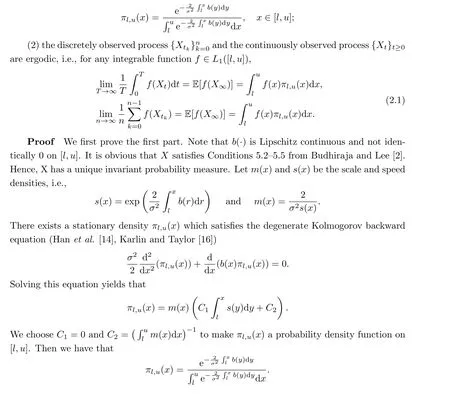
From this,Xhas a unique invariant probability measure,and we can conclude that{Xt}t ≥0 is ergodic (Hanet al.[14]).That the Δ-skeleton{Xtk}nk=0is ergodic follows from Theorem 16.0.1 of Meyn and Tweedie [23].□
The regulatorsLandRin eq.(1.1) are closely related to the local time atlanduof the processX, which will be described in the following lemma.
Lemma 2.2 The regulatorsLandRhave the next representations:
(1) Euler representations.Letn →∞and Δ =T/n →0.For anyandsuch thatl <<<u,N ≤n, andNΔ<t ≤(N+1)Δ, we have that

where [X,X] is the quadratic variation ofX.Using Meyer-Tanaka’s formula (Protter [26]) forYyields that

3 Asymptotic Behavior of the N-W Estimator
In this section, we prove the consistency of the two types of N-W estimators and obtain their asymptotic distributions.
A continuous-type N-W estimator minimizes an objective function
where ˙Mt,forM=X,L,R,denotes the formal derivative ofMwith respect tot.The minimum is achieved at

whereδMtk=Mtk+1-MtkforM=X,L,R.The minimum is achieved at
In order to prove the strong consistency and asymptotic normality of the two types of N-W estimators, we have the following hypotheses:
Hypothesis 2For the continuously observed process,h →0,Th →∞andTh3→0, asT →∞.
Hypothesis 3For the discretely observed process, there exists anεsmall enough such that Δ→0,h →0,nΔ→∞,nhΔ→∞,nh3Δ→0, andnhΔ2-ε →0, asn →∞.
Let
We now state the main results concerning the consistency and the asymptotic normality of the two types of N-W estimators defined in eq.(3.1) and (3.2).
Theorem 3.1Let Hypotheses 1 and 2 hold.Then we have the following results for the continuous-type N-W estimator:
(1)~bT(x) admits the strong consistency, i.e.,

Theorem 3.2Let Hypotheses 1 and 3 hold.Then we have the following results for the discrete-type N-W estimator:
(1)ˆbn(x) admits the strong consistency, i.e.,

while the discrete-type N-W estimator is given by
Remark 3.3The unique invariant density of{Xt}t≥0is given by
With the unique invariant density,similar arguments as to those for the proofs of Theorems 3.1 and 3.2 yield the consistency and asymptotic distributions, so we omit the details here.
Remark 3.4The regulatorLin eq.(3.7) has the following two representations:
(1) the Skorohod representation (Karatzas and Shreve [17]):

4 Numerical Results and Applications
4.1 Numerical Results
In this subsection,we examine and compare the performance of our proposed N-W estimator and the estimator proposed by Cholaquidiset al.[7] (Cholaquidis estimator for short).LetNx= #{0≤k ≤n,Xtk ∈B(x,h)}, where “#” denotes the number of elements in the set.Then the Cholaquidis estimator is defined as
whereI{·}is the indicator function.
We take the diffusion parameterσ=0.2,the initial valuex=0,the lower reflecting barrierl=0, and the upper reflecting barrieru=3.We consider the following three cases:
Case 1b1(x)=sin(2πx)+1.5x;

We plug the different cases ofb(·) into eq.(1.1) and (3.7) to test the numerical behavior of the two estimators.For simulations of reflected SDEs, we make use of the numerical method presented in L´epingle [20], which is known to yield the same rate of convergence as the usual Euler-Maruyama method.
For each setting, we generateN= 1000 Monte Carlo simulations of the sample path,each consisting ofn= 400, 900, and 1600 observations.Based on Hypothesis 3, to obtain N-W estimators with asymptotically negligible bias, we employ Δ=n-2/3and bandwidths in the range (n-0.3,n-0.15).The kernel function we choose is the Epanechnikov kernel, which isK(x)=0.75(1-x2)+,where“+”is the positive part of a real number.Further simulations show that the use of other kernel functions has little impact on the estimator’s empirical performance.We omit the results here.
Let{xi,i= 1,···,300}be the estimated set where the 300 points in the set are taken uniformly from [0,3] to cover the range of the sample path.Two estimators are evaluated by the square-root of average square errors (RASE) for the mean of 1000 estimators, the sample standard deviation (Std.dev), and the median (Median) of 1000 simulations of RASE, where
Tables 1-3 summarize the main results of 1000 simulations.We observe that,as the sample size increases or the bandwidth decreases, the RASE of the two estimators decreases.However,it is obvious that the RASE of the N-W estimator is always much smaller than the Cholaquidis estimator, especially in the case of two-sided barriers.Hence, we conclude that the N-W estimator has a superior performance to the Cholaquidis estimator.
Table 2 Simulation results with a different sample size n and bandwidth h Case 2: b2(x)=
Two-sided N-W estimator Cholaquidis’s estimator n BD(h) RASE Std.dev Median RASE Std.dev Median 400 n-0.15 0.066 0.008 0.077 1.060 0.001 1.060 n-0.2 0.043 0.010 0.063 0.947 0.001 0.948 n-0.3 0.017 0.012 0.068 0.726 0.001 0.728 900 n-0.15 0.060 0.005 0.068 1.020 0.000 1.020 n-0.2 0.037 0.007 0.054 0.883 0.000 0.884 n-0.3 0.013 0.009 0.059 0.642 0.001 0.644 1600 n-0.15 0.055 0.004 0.061 0.983 0.000 0.984 n-0.2 0.032 0.006 0.047 0.838 0.000 0.838 n-0.3 0.010 0.008 0.054 0.594 0.001 0.596 One-sided 400 n-0.15 0.011 0.013 0.043 0.018 0.012 0.042 n-0.2 0.005 0.013 0.051 0.009 0.012 0.047 n-0.3 0.004 0.013 0.068 0.004 0.012 0.063 900 n-0.15 0.009 0.010 0.036 0.014 0.010 0.035 n-0.2 0.004 0.010 0.042 0.007 0.010 0.039 n-0.3 0.002 0.011 0.059 0.003 0.010 0.054 1600 n-0.15 0.007 0.008 0.031 0.011 0.008 0.030 n-0.2 0.003 0.008 0.037 0.005 0.008 0.034 n-0.3 0.002 0.055 0.054 0.002 0.050 0.049
Table 3 Simulation results with a different sample size n and bandwidth h Case 3: b3(x)=2

Table 3 Simulation results with a different sample size n and bandwidth h Case 3: b3(x)=2
Two-sided N-W estimator Cholaquidis’s estimator n BD(h) RASE Std.dev Median RASE Std.dev Median 400 n-0.15 0.061 0.009 0.072 0.836 0.001 0.837 n-0.2 0.044 0.010 0.062 0.742 0.001 0.743 n-0.3 0.025 0.011 0.067 0.566 0.001 0.568 900 n-0.15 0.054 0.006 0.062 0.802 0.000 0.802 n-0.2 0.039 0.007 0.054 0.693 0.001 0.694 n-0.3 0.020 0.009 0.058 0.500 0.001 0.503 1600 n-0.15 0.050 0.005 0.057 0.776 0.000 0.776 n-0.2 0.035 0.006 0.048 0.657 0.000 0.658 n-0.3 0.018 0.007 0.052 0.463 0.001 0.465 One-sided 400 n-0.15 0.055 0.010 0.069 0.075 0.009 0.084 n-0.2 0.041 0.010 0.064 0.057 0.009 0.073 n-0.3 0.024 0.011 0.069 0.032 0.010 0.068 900 n-0.15 0.049 0.008 0.060 0.067 0.007 0.074 n-0.2 0.036 0.007 0.054 0.048 0.007 0.061 n-0.3 0.019 0.009 0.060 0.026 0.008 0.058 1600 n-0.15 0.045 0.006 0.053 0.061 0.005 0.067 n-0.2 0.032 0.006 0.047 0.043 0.005 0.054 n-0.3 0.017 0.007 0.053 0.023 0.007 0.051
Figures 1-3 represent the two estimators from the three cases withn=1600 andh=n-0.3in the interval [0,3].For the case of two-sided barriers, the N-W estimator shows competitive performance compared to the Cholaquidis estimator in the interior.However, in the area near barriers 0 and 3,the N-W estimator has a remarkably better performance than the Cholaquidis estimator.Hence, the RASE of the Cholaquidis estimator is much bigger than the N-W estimator due to the bad performance in the area near the two barriers.For the case of a one-sided barrier, the N-W estimator also has better performance than the Cholaquidis estimator.

Figure 1 b(x)=sin(2πx)+1.5x with two-sided reflecting barriers(left)and a one-sided barrier(right),where “CE” is Cholaquidis estimator, “NWE” is the N-W estimator, and “True” is the true value of the function b(x)

Figure 2 b(x)= with two-sided reflecting barriers (left) and a one-sided barrier (right)

Figure 3 b(x)=ith two-sided reflecting barriers (left) and a one-sided barrier (right)
4.2 Applications to Currency Exchange Rates
In the preceding discussion we presented an efficient estimation procedure for the drift function of a reflected SDE.The interesting idea of applying reflected SDEs to target zone models of currency exchange rates was proposed by Bertola and Svensson [1] and Krugman[18].Actually, government regulations result in spot foreign exchange rate processes being constrained(with lower and upper barriers)in a regulated financial market.This suggests that using reflected SDEs as dynamic models is appropriate, as that is consistent with financial dynamics in reality (Boet al.[3]).
We consider currency exchange rates based on the data sets from the People’s Bank of China and the Federal Reserve Board.We show the daily foreign exchange rate processes for four assets including USD/CNY, EUR/CNY, AUD/CNY and EUR/USD, all of which are collected from 2002-01-01 to 2022-09-20(see Figure 4).We adopt the convention that the equal time interval for the “daily” interest rates is Δ = 0.042, while one unit of time represents one month.The bandwidth we select isn-0.3, wherenis the total number of observations.
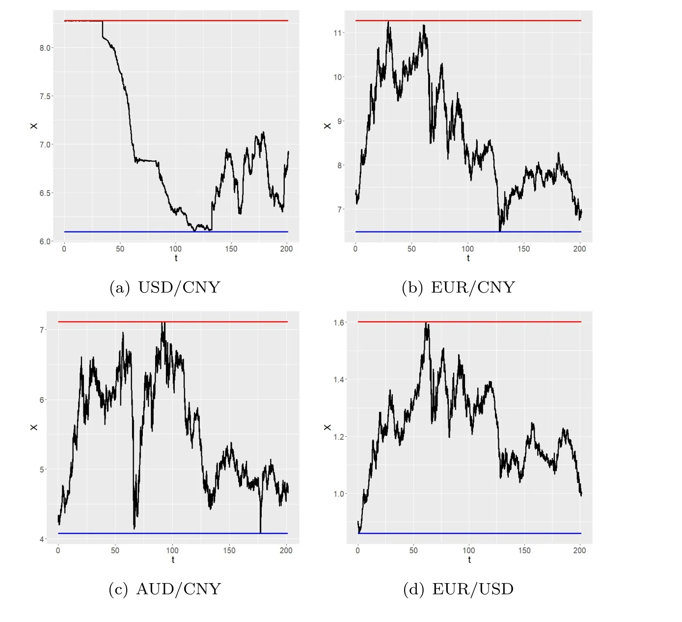
Figure 4 Daily currency rate (solid black line) with the horizontal blue line being the lower reflecting barrier and the horizontal red line being the upper reflecting barrier
Figure 5 displays the N-W estimators for the drift function of the four currency exchange rate processes.The estimator of the drift function is reasonable in its interior, while the confidence intervals around the barriers are generally much wider, due to a lack of data around the barriers (see Figure 5).This is also the disadvantage of N-W estimators (Fan and Gijbels[8]).

Figure 5 The N-W estimators (the solid black line) for the drift function of daily currency rate processes with the red and blue dashed lines demonstrating the confidence interval
5 Proofs of the Main Results
In this section, we give the proofs of Theorems 3.1 and 3.2.We first introduce a useful alternative expression for the discrete-type N-W estimator.Note that

An alternative expression for the discrete-type N-W estimator ˆbn(x) turns out to be

For the convenience of the discussion to follow, we define that


Proof of Claim (C2)SinceKis bounded and integrable on [l,u], by the dominated convergence theorem and Itˆo’s isometry, we have that

whereC1is a constant.This follows immediately becauseGT,2(x) converges to, a Gaussian random variable with a mean of 0 and a varianceC1(Th)-1for theFt-adapted processXasT →∞.For anyt >0, we define the integerτtbyτt ≤t <τt+1.For anyε >0 and a positive integerpbeing large enough, using Chebyshev’s inequality yields that
Hence, the second term of eq.(5.2) is equal to 0.By the Lipschitz continuous ofb(·), we have
that
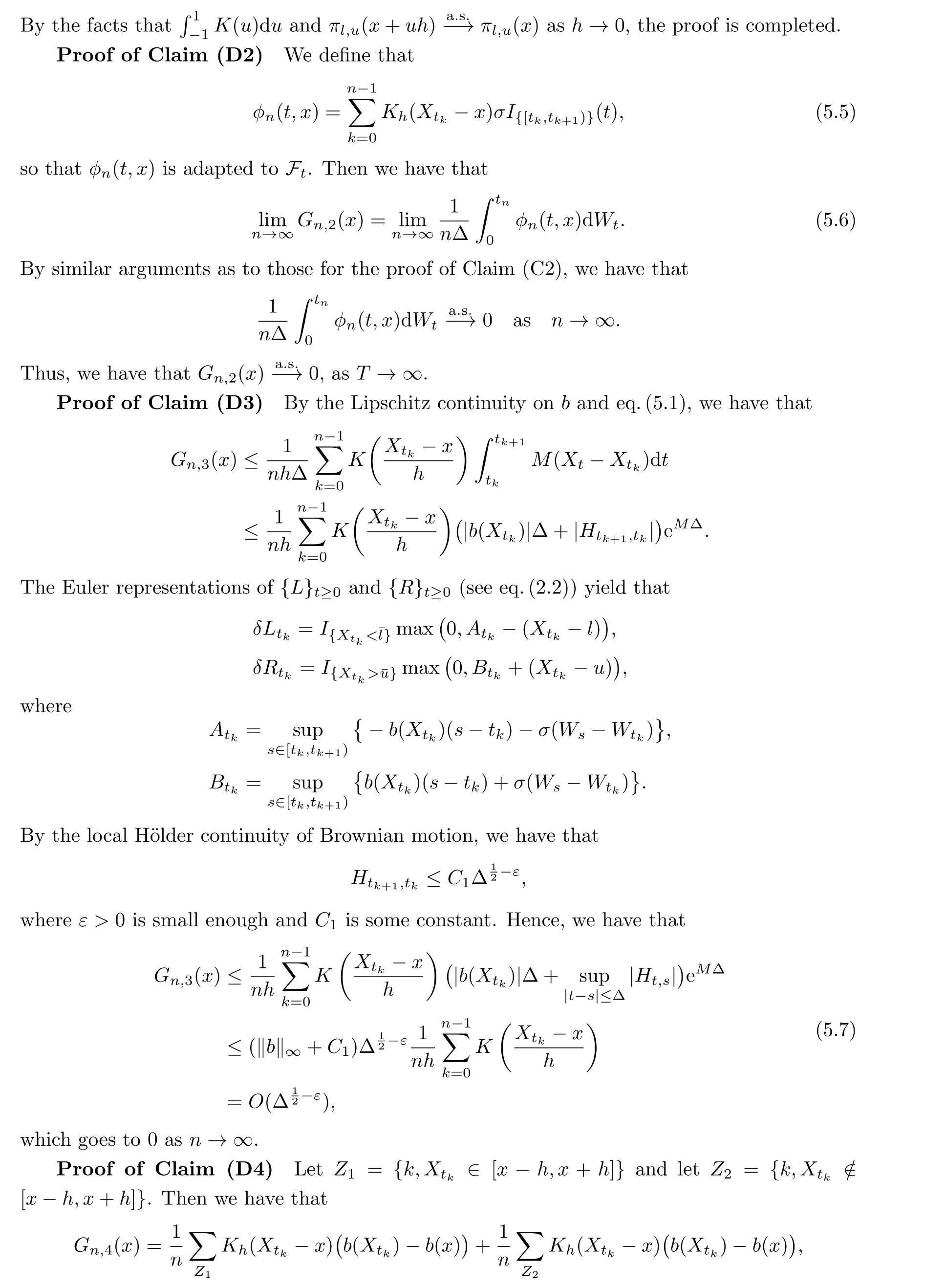
where the second term is equal to 0.By the Lipschitz continuity ofb(·), we have that
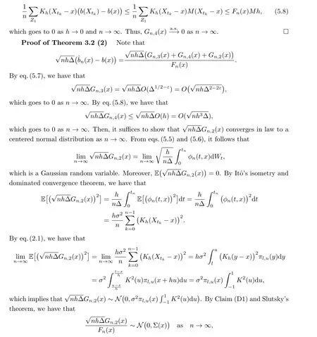
which completes the proof.□
Conflict of InterestThe authors declare no conflict of interest.
杂志排行
Acta Mathematica Scientia(English Series)的其它文章
- THE EXACT MEROMORPHIC SOLUTIONS OF SOME NONLINEAR DIFFERENTIAL EQUATIONS*
- GLOBAL CLASSICAL SOLUTIONS OF SEMILINEAR WAVE EQUATIONS ON R3×T WITH CUBIC NONLINEARITIES*
- SOME NEW IDENTITIES OF ROGERS-RAMANUJAN TYPE*
- QUASIPERIODICITY OF TRANSCENDENTAL MEROMORPHIC FUNCTIONS*
- THE LOGARITHMIC SOBOLEV INEQUALITY FOR A SUBMANIFOLD IN MANIFOLDS WITH ASYMPTOTICALLY NONNEGATIVE SECTIONAL CURVATURE*
- GLOBAL SOLUTIONS TO 1D COMPRESSIBLE NAVIER-STOKES/ALLEN-CAHN SYSTEM WITH DENSITY-DEPENDENT VISCOSITY AND FREE-BOUNDARY*
