Superiority of a Convolutional Neural Network Model over Dynamical Models in Predicting Central Pacific ENSO

Tingyu WANG and Ping HUANG

1Center for Monsoon System Research, Institute of Atmospheric Physics,Chinese Academy of Sciences, Beijing 100029, China

2Collaborative Innovation Center on Forecast and Evaluation of Meteorological Disasters (CIC-FEMD),Nanjing University of Information Science & Technology, Nanjing 210044, China

3State Key Laboratory of Numerical Modeling for Atmospheric Sciences and Geophysical Fluid Dynamics,Institute of Atmospheric Physics, Chinese Academy of Sciences, Beijing 100029, China

4University of Chinese Academy of Sciences, Beijing 100049, China

ABSTRACT The application of deep learning is fast developing in climate prediction,in which El Niño–Southern Oscillation(ENSO),as the most dominant disaster-causing climate event,is a key target.Previous studies have shown that deep learning methods possess a certain level of superiority in predicting ENSO indices.The present study develops a deep learning model for predicting the spatial pattern of sea surface temperature anomalies (SSTAs) in the equatorial Pacific by training a convolutional neural network (CNN) model with historical simulations from CMIP6 models.Compared with dynamical models,the CNN model has higher skill in predicting the SSTAs in the equatorial western-central Pacific,but not in the eastern Pacific.The CNN model can successfully capture the small-scale precursors in the initial SSTAs for the development of central Pacific ENSO to distinguish the spatial mode up to a lead time of seven months.A fusion model combining the predictions of the CNN model and the dynamical models achieves higher skill than each of them for both central and eastern Pacific ENSO.

Key words: ENSO diversity,deep learning,ENSO prediction,dynamical forecast system

1.Introduction

El Niño–Southern Oscillation (ENSO) is the most important sea surface temperature anomaly (SSTA) signal in global climate anomalies because of the changes in atmospheric circulation it generates (Ashok et al.,2007;Weng et al.,2007;Yang and Huang,2021).In particular,the locations of SSTA centers during ENSO are crucial in the occurrence of climate anomalies globally (Weng et al.,2007;Kim et al.,2009;Wang and Wang,2014).The spatial pattern of ENSO varies by event,with the location of the center varying from the warm pool to the coast of America,which impacts the regional climate in a distinct way (Larkin and Harrison,2005;Ashok et al.,2007;Weng et al.,2007;Rodrigues et al.,2011,2015;Patricola et al.,2016).For convenience,the spatial pattern of ENSO is often classified into two-types,known as the central Pacific (CP) type with SSTAs centered near the date line,and the eastern Pacific (EP) type with SSTAs centered near the eastern equatorial Pacific (Kao and Yu,2009;Kug et al.,2009),although the centers of all ENSO cases are not discretely clustered into these two locations (Capotondi et al.,2015).CP ENSO has been occurring more frequently since the late 20th century (Yeh et al.,2009;Lee and McPhaden,2010;Newman et al.,2011;Freund et al.,2019),so improving our ability to predict this particular type of event has become increasingly urgent.

The amplitude of CP ENSO is comparatively smaller than that of EP ENSO,both in observations and models(Capotondi et al.,2015),and the key process in its development–namely,zonal advection–is closely connected with the atmospheric zonal wind.Moreover,the signal-to-noise ratio of CP El Niño is similar compared to the surface zonal wind (Capotondi et al.,2020).Thus,although there is a higher predictability in the central Pacific than the eastern Pacific (Kim et al.,2009),CP ENSO is relatively harder to predict in dynamical models (Imada et al.,2015;Zheng and Yu,2017),especially during boreal winter (Jeong et al.,2012).Specifically,current state-of-the-art dynamical models cannot accurately predict the central location of ENSO events for lead times longer than one month (Hendon et al.,2009;Ren et al.,2019;Capotondi et al.,2020).Therefore,identifying the central locations of ENSO events,especially for CP ENSO,remains a great challenge in ENSO prediction.

Deep learning is a method that has been applied in many fields during the last decade (Deng and Yu,2014;Xu et al.,2021;Taylor et al.,2022;Wang et al.,2023),but it is still difficult to apply in seasonal climate prediction because the climatic observational record is not long enough to support big-data training,which is often required in deep learning methods (Hirahara et al.,2014).Recently,the vast model datasets from phase 5 of the Coupled Model Intercomparison Project (CMIP5) were used to train a convolutional neural network (CNN) for predicting the ENSO index,which obtained a higher prediction skill than dynamical climate models (Ham et al.,2019).Since then,the application of deep learning methods in climate science has been gaining increasing recognition (Tang and Duan,2021;Boschetti et al.,2022;Shin et al.,2022).The success of the CNN method based on the outputs of CMIP dynamical models indicates that dynamical models have great potential in ENSO prediction,although a previous study (Newman and Sardeshmukh,2017) revealed that the direct predictions of dynamical models do not show superiority compared with a simpler linear reverse model constructed from observations.

As most CNN models are applied to predict one-dimensional indices of ENSO (Broni-Bedaiko et al.,2019;Pal et al.,2020;Yan et al.,2020;Cachay et al.,2021),these previous deep learning models for ENSO prediction are not designed for predicting the spatial pattern of ENSO–especially its central location.A single index cannot distinguish well the spatial type of ENSO,although CP ENSO events are often related to modest or weak El Niño and strong or moderate La Niña events,and EP ENSO events to strong El Niño and weak La Niña events.By evaluating the predicted El Niño categories,Ham et al.(2019) suggested the CNN method shows a higher hit rate for the type of ENSO than North American Multi-Model Ensemble (NMME) models,but spatial pattern information was lacking.Therefore,it is urgent to develop a new method to explicitly predict the twodimensional SSTA,which would be able to identify the types of upcoming ENSO events more directly.

Here,we use the historical simulations from 39 state-ofthe-art CMIP6 models to train CNN models for predicting the leading principal components of the tropical Pacific SSTAs,which can reconstruct the SSTAs two-dimensionally.Evaluation of the predicted two-dimensional SSTAs indicates that the deep learning model outperforms current dynamical models in predicting CP ENSO.

The remainder of this study is organized as follows:The dataset used and the training and attribution details of the CNN model are introduced in section 2.The prediction skill of the CNN model and fusion model are evaluated and analyzed in section 3.We provide conclusions and point out some limitations of this model in section 4.

2.Data and methods

2.1.Deep learning model

In the deep learning model developed for the present study,we utilize the SSTAs at the initial time and the SSTA tendency (55°S–70°N,0°–360°E),defined by the difference between the SSTA in the initial month and that at a twomonth lead,as the predictors (Ham et al.,2019;Wang et al.,2020).The SSTA tendency includes the signals of SSTA evolution and ocean dynamics (Enfield and Mayer,1997;Lau and Nath,2003;McPhaden,2012),which replaces upper ocean heat content anomalies often used in previous studies(Ham et al.,2019;Feng et al.,2022).

To forecast the two-dimensional structure of SSTAs,we first train our CNN model to predict the principal components of three leading empirical orthogonal function (EOF)modes of the tropical Pacific,and then reconstruct the predicted coefficients into two-dimensional SSTAs with the predefined EOF modes.We select the three leading EOF modes of the observed SSTAs in the tropical Pacific (10°S–10°N,120°E–80°W),and the period from 1960 to 1986 to avoid future information leaking into the prediction system,which together can explain around 87% of the total SSTA variance [Fig.S1 in the electronic supplementary material(ESM)].Comparison of the prediction skills of commonly used CNN models (Fig.1) suggests that the VGG-11 model has obvious advantages for the present study,and thus this model is selected.Further details on the reason for choosing the VGG-11 model,the EOF decomposition and reconstruction,and other aspects of training the CNN model,can be found in section 2.3.

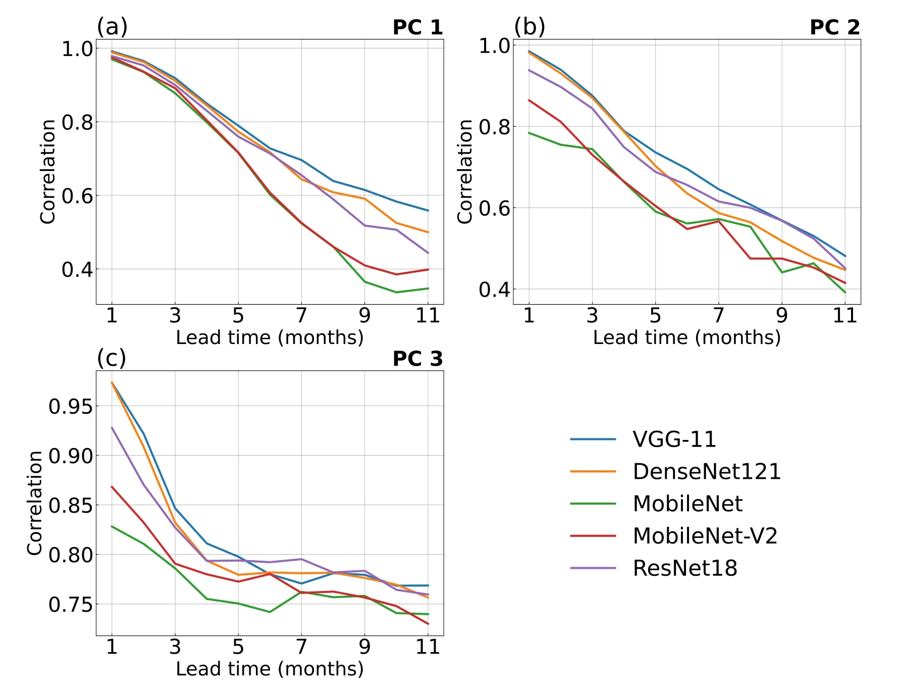
Fig.1.Prediction skill comparison in the principal components of three leading EOF modes [(a) PC1,(b)PC2,and (c) PC3] among five commonly used CNN models: VGG-11 (blue line),MobileNet-V2 (red line),DenseNet121 (yellow line),ResNet18 (purple) and MobileNet (green line).

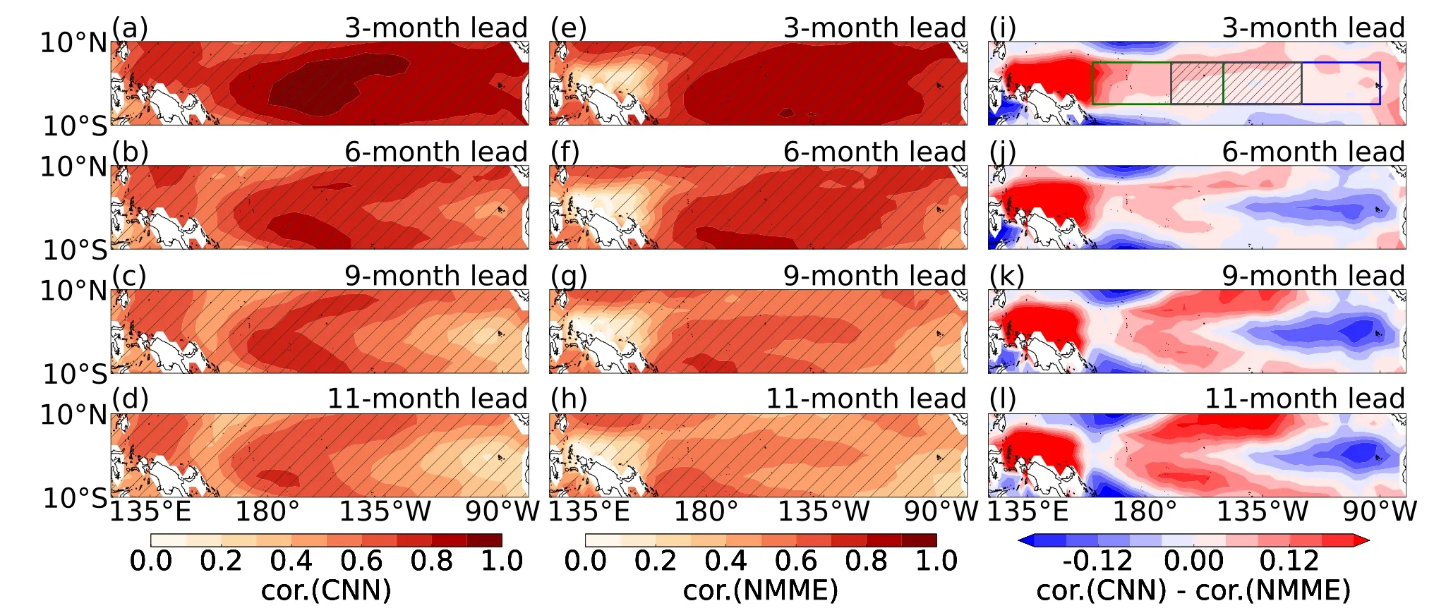
Fig.2.Prediction skill for the SSTAs in the equatorial Pacific.Prediction skill of the (a–d) CNN model and (e–h) NMME models at 3-,6-,9-and 11-month leads.Stippled regions are statistically significant at the 5% level.(i–l) Difference in the prediction skill of the CNN model from the MME of the dynamical models participating the NMME project.The Niño-3,Niño-4 and Niño-3.4 regions are indicated by the blue,green and stippled boxes in (i),respectively.The validation period is 1986–2019.

2.2.CMIP6 datasets, observations and NMME models

The historical simulations of 39 climate models participating in CMIP6 (Eyring et al.,2016) for the period 1948–2014 are used to train the CNN model [Table S1 in the electronic supplementary material (ESM)].Previous studies have concluded that CMIP6 models offer considerable improvements in simulating the properties of ENSO relative to their CMIP5 counterparts (Eyring et al.,2019;Zelinka et al.,2020).The data during the period 1984–2009 are used to calculate the climatology and anomalies.Then,the SSTAs in all CMIP6 models are projected onto the three observed EOF modes,and the projection coefficients are treated as the predictands for training the CNN model.The monthly COBE-SST2 dataset (Hirahara et al.,2014) from 1984 to 2019 is used as the observation to provide the initial values,validate the prediction skill,and develop the fusion model.To compare with the prediction skill of the CNN model,the prediction results of six NMME models (Table S2 in the ESM) from 1986 to 2019 are also used (Kirtman et al.,2014),which represent the state-of-the-art in dynamical models for ENSO prediction.The NCEP-CFSv2 model is excluded in calculating the MME because of its short lead time.We also evaluated the skills between the CNN and MME of dynamical models for a shorter lead time by adding NCEP-CFSv2,and found no considerable change in skill (Fig.S2 in the ESM).All datasets are interpolated to a 2.5° × 2.5° spatial resolution,and the temporal signal below three months is removed using a Butterworth filter for comparison with previous studies.The result using the Butterworth filter is similar to that of the running average,so does not influence the conclusions.

2.3.Predictions of two-dimensional SSTAs in the tropical Pacific

The CNN model can capture the teleconnection of ENSO well (Ham et al.,2019),and is suitable to the limited sample size of the CMIP6 simulation dataset.Some architectures of CNN models,such as UNet,can predict spatial fields (Prabhat et al.,2021).Taylor and Feng (2022)achieved improvement in two-dimensional SST prediction using UNet-LSTM,but our preliminary study (not shown)indicates that a neural network with the UNet encoder–decoder module is not suitable for identifying the central location of ENSO.Thus,the CNN method with the one-dimensional output is selected in the present study to construct the deep learning model for ENSO prediction.To fit the onedimensional output of the CNN model,we first predict the coefficients of three leading spatial modes of the tropical Pacific SSTAs,and then reconstruct two-dimensional patterns of SSTAs by using corresponding EOF modes.

The leading spatial modes of the tropical Pacific SSTAs are extracted by EOF analysis performed on the observed SSTAs in the equatorial Pacific for the period from 1960 to 1986 (10°S–10°N,120°E–80°W) (Wilks,2019).We select the first three EOF modes (Fig.S1),which explain 86.65% of the total SSTA variance,almost all largescale interannual variabilities,and are unbiased to any types of ENSO (Takahashi et al.,2011).We choose the mean square error as the cost function and train the CNN model through iteration to minimize the error between the prediction and the true coefficients.An individual model is trained to optimize each coefficient.The projection coefficients of the SSTAs in CMIP6 models and in the CNN model output are normalized to have a mean of 0 and a standard deviation of 1.

We preliminarily test five commonly used CNN models–namely,VGG-11 (Simonyan and Zisserman,2015),MobileNet,MobileNet-V2 (Sandler et al.,2018),DenseNet121 (Huang et al.,2017) and ResNet18 (He et al.,2016)–in the prediction with the same hyperparameters.The VGG-11 model is selected for further study because of its obvious advantages among the five models (Fig.1).The VGG-11 model (Simonyan and Zisserman,2015) is a classic CNN model with simple architecture composed of a 3 × 3 grid convolutional filter,pooling,and ReLU activation function (Fig.S3 in the ESM).The VGG-11 model has the smallest network capacity,i.e.,model layers and number of parameters in the hidden layers,compared to the other four models,which prevents the problem of overfitting (Fig.1).On the other hand,the larger training data spatial resolution (2.5° ×2.5°) used in the present study provides a larger network capacity than previously (Ham et al.,2019).Activation functions,such as Sigmoid,tanh and ReLU play a critical role in introducing nonlinearity to CNN models.

The ReLU function is included in the present CNN model,which is used to predict the coefficients of the three EOF modes one year ahead.We train 33 CNN submodels individually for the 11 lead months and three coefficients of EOF modes as an ensemble member.In order to eliminate the impacts of the initialized model weights on training,we train 10 members with slightly different and random initialized weights,and then the ensemble results of the 10 members are treated as the results of the prediction.The hyperparameters in the VGG-11 model are set as: mini-batch size=128;epoch number=35;initial learning rate=0.0001;warm-up training schedule used in the first five epochs;and stochastic gradient descent with momentum for the optimizer.Batch normalization is applied for faster and more stable training.An early stop training strategy is used to prevent overfitting of the model.

After the coefficients for the EOF modes have been predicted at a certain lead time,we can reconstruct the twodimensional pattern of SSTAs using the predicted coefficients and the associated EOF modes.Then,the reconstructed twodimensional SSTAs serve as the final prediction for the tropical Pacific SSTAs at that lead time.There is no transfer learning applied in the present CNN model,which makes it different from previous linear reverse models based on observations (Newman and Sardeshmukh,2017).The skill of the predicted SSTAs is evaluated with the full SSTA of the observation.

2.4.Zonal SSTA center during ENSO

To further evaluate the prediction skill for the pattern of SSTAs during CP and EP ENSO events,we calculate the zonal SSTA center during the four types of ENSO events,i.e.,EP El Niño,CP El Niño,EP La Niña,and CP La Niña.Although the spatial differences between the EP and CP La Niñas are not as apparent as those between the EP and CP El Ninos,the La Niñas are still divided into two types owing to the overall differences in amplitude,evolution,precursor,and location (Capotondi et al.,2015).These events are distinguished by modifying a unified complex ENSO index (UCEI) (Zhang et al.,2019):

in whichN3andN4denote the Niño-3 and Niño-4 indices,respectively.EP La Niña is defined for-180◦<θ<-90◦;CP La Niña is defined for-270◦<θ<-180◦;EP El Niño is defined for 0◦<θ<90◦,while CP El Niño is defined for-90◦<θ<0◦.The classification of ENSO events is shown in Table 1.

Table 1.CP El Niño,EP El Niño,CP La Niña,and EP La Niña events during 1986–2019.

Then,we calculate the zonal center location of the equatorial (averaged within 5°S–5°N) profiles of the predicted Pacific SSTA for the four types of events.The zonal center location is defined as the longitude with the maximum of the zonal SSTA profiles for the positive events and the minimum for the negative events,and a three-point moving average is applied to the zonal profile of SSTAs.The composite locations are evaluated because it is hard to distinguish a single center in one individual event owing to the small-scale variations.As shown in Fig.S4 in the ESM,however,the NMME models cannot predict the large-scale pattern of SSTAs for some events at a long lead time.For example,the CNN model correctly forecasts the 1994/95 boreal winter as CP El Niño,whereas the NMME models forecast a La Niña event (Fig.S4a in the ESM).In this case,there is actually not a real center for the predicted SSTAs.Thus,we exclude the predictions with low skill for the large-scale pattern of SSTAs before evaluating the center location.The predictions whose pattern correlations with the observed SSTAs are less than 0.3 are replaced by the average center of other events at each lead time.The percentages of the selected events in calculating the zonal centers for each lead month are shown in Tables S3 and S4 in the ESM.The bootstrap method is used to estimate the confidence level of the composite prediction.In consideration of the small number of cases in each type,we randomly sample the center location from each ENSO type,and each time a new set of samples is obtained.The mean of the center location of this set of samples is calculated and considered to be the composite center position of the new samples.This operation is repeated 1000 times to obtain a distribution of ENSO center positions of this type,and the values of the 5% and 95% quartiles from the distribution are selected as confidence intervals.

2.5.Integrated gradients for attribution of the CNN model’s prediction

The integrated gradients method (Sundararajan et al.,2017) is used in this study to attribute the prediction of the CNN model.Given an SSTA input X,the functionF(X) representing the CNN model is a highly nonlinear function of X.The CNN modelF(X) can be approximated with a linear function by using first-order Taylor expansion:F(X)≈ωTX+b.Then,the gradients ω for each grid point(i,j) in X can be calculated as

Here,the integrated gradients for each grid point of the SSTA fields are calculated using the Captum Python package(Kokhlikyan et al.,2020).

Since the third EOF mode is mainly associated with the warming trend in the equatorial Pacific,which shows a slight influence on the prediction skill,the integrated gradients for the coefficients of the two leading EOF modes are calculated and added together as the result to show in the heat map,representing the estimated contribution of the initial SSTAs to the prediction of the CNN model.We scale the result in each grid point by the maximum absolute value,leading to a unitless heat map.Although a previous study illustrated that the integrated gradient method has some limitations to explain the results of the deep learning method(Mamalakis et al.,2022),it can still track down the smallscale,midlatitude signals that appear one year ahead.

2.6.A fusion model combining the dynamical models and deep learning model

Considering the respective advantages of the dynamical models and the CNN model in the eastern and central Pacific,we develop a fusion model combining their predictions.The fusion model combines the predictions from the two types of models in each lead month and grid point as follows:

3.Results

3.1.Prediction of tropical Pacific SSTAs

Using the trained CNN model,we run the prediction for the period 1986–2019.Figure 2 shows the correlation skill of the predicted SSTAs and compares the prediction skill with state-of-the-art dynamical models participating in the NMME project (Kirtman et al.,2014).The highest prediction skill of the present CNN model is located in the equatorial central Pacific (Figs.2a–d),with the all-season correlation coefficient reaching up to about 0.7 at a lead time of around one year,which is consistent with the result in Taylor and Feng (2022).The pattern of prediction skill of the NMME dynamical models (Figs.2e–h) is similar to that of the CNN model,with the highest skill in the central Pacific,which is consistent with the result in Kim et al.(2009).By contrast,the different skills between the central and eastern Pacific in the NMME models are much weaker than that in the CNN model.The apparently lower prediction skill of the CNN model in the eastern Pacific could be due to the fact that CNNs are better at finding nonlinear mappings for processes poorly described by physical laws and parameterizations(Irrgang et al.,2021),but the SSTAs in the eastern Pacific are often dominated by thermocline dynamical processes(Zheng and Yu,2017;Capotondi et al.,2020).

Comparing the skill between the CNN model and the NMME models,we find a nonuniform advantage of the deep learning method relative to the NMME dynamical models (Figs.2i–l),although previous studies have demonstrated that CNN models possess apparent advantages in predicting the Niño-3.4 index (Ham et al.,2019).The obvious advantages of the CNN model are mainly located in the equatorial western and central Pacific,but not in the Niño-3.4 region(Figs.2i–l).The advantage of the CNN model in the central Pacific increases along with lengthening of the prediction lead time.The all-season correlation coefficient of the CNN model at a one-year lead time is around 0.2 larger than that of the NMME models in most regions.By contrast,the NMME dynamical models show some advantages over the CNN model in the equatorial eastern Pacific from a lead time of around six months (Figs.2i–l).

Comparison between the CNN model and the NMME models illustrates that the advantage of the CNN model is mainly located in regions with a lower amplitude of SSTA variability,possibly because the SSTAs in these regions are more sensitive to external forcing (Imada et al.,2015).On the other hand,the advantages of the dynamical models are mainly located in the eastern Pacific,where ocean dynamics dominates the SSTA variability (Kao and Yu,2009;Zheng and Yu,2017).The higher prediction skill of the CNN model in the central Pacific implies that the CNN model will have higher skill in predicting CP ENSO than EP ENSO.

As the three leading modes of the tropical Pacific SSTAs are able to describe some variabilities of the longterm trend,the improvement of the CNN model in the western and central Pacific could be artificially induced by the consistent warming trend of the warm pool regions in the CMIP6 historical simulations and the observation.To clarify this point,we also train another CNN model with detrended CMIP6 historical simulations,and use the detrended observation data as the validation.The result (Fig.S5 in the ESM)of the new CNN model also exhibits apparent improvement in the equatorial western and central Pacific,which excludes the potential role of the consistent warming trend in the training and validation datasets.

3.2.Skill in predicting CP and EP ENSO index

The prediction skills of the CNN model for the two types of ENSO are evaluated based on two ENSO indices:the warm-pool index (WPI) and cold-tongue index (CTI)(Ren and Jin,2011).These two indices are linear combinations of the Niño-3 and Niño-4 indices but uncorrelated with each other (Text S1 in the ESM).Figure 3a shows the all-season correlation skills of WPI and CTI from 1986 to 2019.For the WPI related to CP ENSO projected by the NMME models,a correlation coefficient above 0.6 at a lead time of up to nine months is only achieved by CanCM4i and the MME,whereas the skill of the CNN model for the WPI is systematically superior to all NMME models and their MME at all lead months.On the contrary,the skill of the CNN model for the CTI related to EP ENSO (Fig.3b)decreases apparently after the first four lead months,which is lower than the skills of some of the dynamical models.Figure 4 shows the season-dependent prediction skill for the ENSO indexes simulated by the CNN model and the NMME models.The season-dependent and season-independent index predictions both demonstrate that there is a greater superiority of the CNN model in predicting CP ENSO.

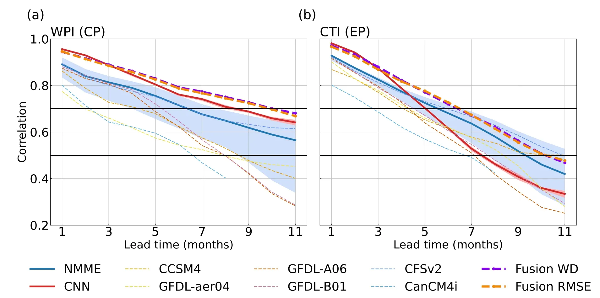
Fig.3.All-season prediction skill for the two types of ENSO in the CNN model.(a) Prediction skill for CP ENSO,represented by the warm-pool index,as a function of the forecast lead month in the CNN model (red),the individual dynamical models in the NMME project,and their ensemble.(b) As in (a) but for the skill of EP ENSO,represented by the cold-tongue index.The shading around the lines of the CNN and the MME represents the 95% confidence interval using the bootstrap method.The purple and orange dashed curves denote the prediction skill of the fusion model based on Wasserstein distance and RMSE,respectively.The validation period is 1986–2019.

Fig.4.Prediction skill of ENSO indices depending on season: (a,b) CP ENSO and (c,d) EP ENSO predicted by (a,c) the CNN model and (b,d) the NMME models.Correlation coefficients less than 0.6 are masked.

3.3.Prediction of the SSTA pattern during ENSO events

Another key indicator of the skill of the CNN model in predicting ENSO SSTAs is whether it can distinguish between the spatial modes of ENSO.To test this,we select ENSO events during 1986–2019 based on the boreal winter(December–February;DJF) SSTAs in which the DJF-averaged Niño-3.4 index is greater than 0.5°C or less than-0.5°C.These events are then divided into CP El Niño,EP El Niño,CP La Niña,and EP La Niña (Table 1) (Capotondi et al.,2020).The prediction skill for the SSTA pattern during ENSO events in the CNN model and the NMME models is measured by the pattern correlation coefficient (Fig.5 and Fig.S4 in the ESM).As shown in Fig.5a,the CNN model has apparent superiority in predicting most CP ENSO events at lead times of four to eleven months relative to the NMME models.Moreover,the CNN model successfully forecasts the double-dip CP La Niña events one year ahead from 2010 to 2012 (Fig.S4 in the ESM).By contrast,for EP ENSO events,the skill of the CNN model is not higher than the dynamical models,except for the 2017/18 event(Fig.5b).This pattern correlation result for the two types of ENSO cases is consistent with the evaluation based on the two indexes that the superiority of the CNN model is mainly in forecasting CP ENSOs rather than EP ENSOs.

Fig.5.Different prediction skill between the CNN model and the NMME models for the spatial pattern of the two types of ENSO events [(a) CP ENSO;(b) EP ENSO] in the DJF season from 5-to 11-month leads.The prediction skill in each lead month is measured by the pattern correlation.

The zonal centers of the predicted SSTAs during the four ENSO types are also further evaluated,which are defined as the longitude with the maximum of the composited equatorial SSTA profiles for the positive events and the minimum for the negative events (section 2.4).The CNN model can predict the locations of the zonal SSTA centers of CP El Niño events closer to the observation than the NMME dynamical models in all lead months (Fig.6a);whereas,for EP El Niño events,the CNN model can predict the centers skillfully at lead times of one to seven months,and better than the NMME models at lead times of up to five months (Fig.6b).Comparing Fig.6a and Fig.6b,we can see that the NMME dynamical models tend to predict all El Niño events as EPtype events,albeit with some distinction but only at a onemonth lead,as is the case for most other dynamical models(Ham and Kug,2012).However,by contrast,the CNN method is able to distinguish between the spatial modes of ENSO at a seven-month lead because of its high skill with respect to the zonal SSTA centers of CP El Niño events.For La Niña events,the CNN model has obvious superiority relative to the NMME dynamical models for CP La Niña events at lead times of one to nine months,as well as for EP La Niña events at lead times of three to four months.Both for CP El Niño and La Niña,the NMME models cannot simulate well the westward extension of the CP-type SSTAs,resulting in a less skillful forecast than the CNN model.

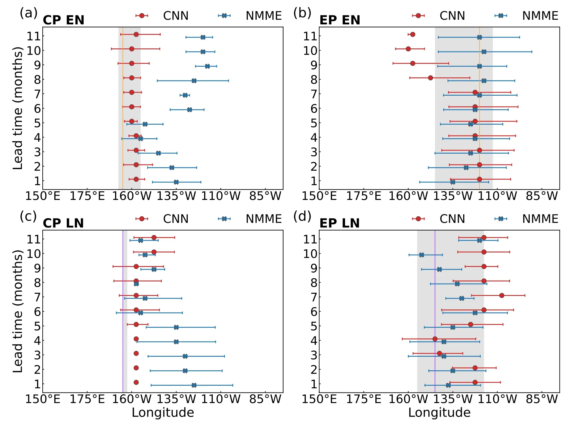
Fig.6.Prediction of the zonal SSTA center for different ENSO types: (a–d) zonal centers of the SSTAs during (a)CP El Niño,(b) EP El Niño,(c) CP La Niña,and (d) EP La Niña,projected by the CNN model (red dots) and the NMME models (blue crosses).The error bars indicate the 90% confidence interval from the bootstrap method.The vertical lines indicate the composite zonal centers in the observations,and the vertical shading represents the 90%confidence interval of the composite based on the bootstrap method.

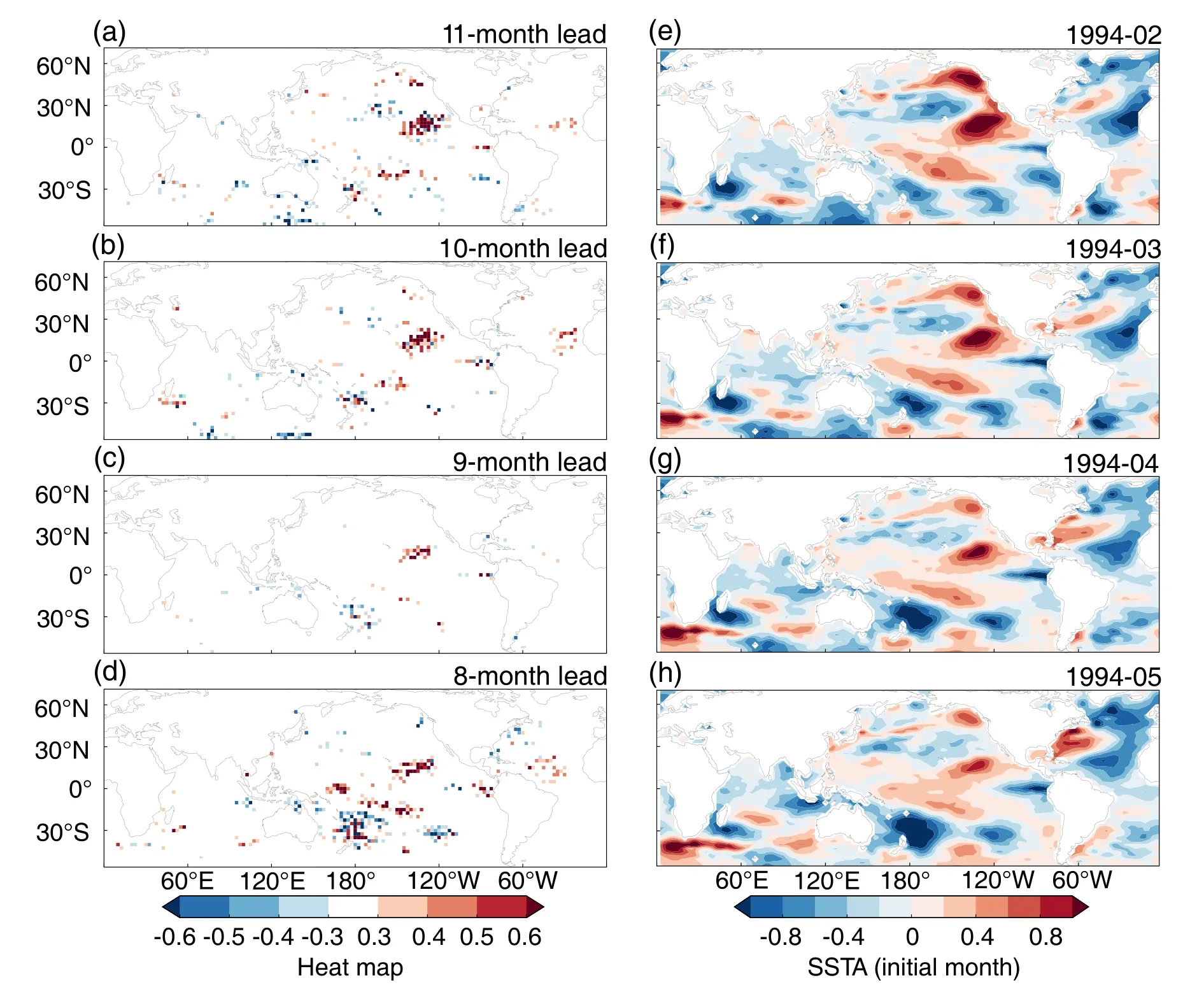
Fig.7.Dynamic attribution of the CNN model in predicting the 1994/95 CP ENSO event.Different initial months are used to predict the January 1995 CP El Niño: (a–d) heat map for the initial months of February,March,April and May 1994;(e–h) SSTAs of February,March,April and May 1994 used to predict equatorial Pacific SSTAs in January 1995.

3.4.Attribution of the CNN model’s prediction

The integrated gradients method is applied to understand what the CNN model has learned from the input data in predicting the spatial mode of ENSO well (section 2.5) (Toms et al.,2020).The integrated gradients method has been proven to be more sensitive to most signals (Sundararajan et al.,2017) compared with other gradients-based methods(Baehrens et al.,2010;Simonyan et al.,2014) used in previous attribution studies for deep learning models.In short,the integrated gradients method estimates the contribution of the initial SSTAs to the prediction of the CNN model,and the degree of contribution can be shown numerically on a heat map.The attribution heat map can highlight the most decisive signals in the input SSTAs for the prediction.Furthermore,positive (negative) values over a certain region denote that they make a positive (negative) contribution to the prediction.We generate a heat map using the integrated gradients method for the prediction of a case,the 1994/95 CP El Niño event.As shown in Fig.5,the CNN model shows apparent superiority compared with the NMME for the 1994/95 CP El Niño.The CNN model successfully forecasts it as a CP El Niño event one year ahead,while the dynamical models forecast it as a cold event (Fig.S4 in the ESM).February,March,April and May 1994 are each selected as the initial month,at leads of eight to eleven months,to forecast the SSTAs in the target month of January 1995.

Figures 7a–d show the heat maps for the initial SSTAs in February–May 1994,respectively.There are two apparent signals in the heat maps,which are the precursors recognized by the CNN model in predicting the 1994/95 CP El Niño.One is the Northeast Pacific Ocean between Hawaii and Baja California with warm SSTAs,appearing as a Pacific meridional mode (Chiang and Vimont,2004).These warm SSTAs extend and persist southwestward over the following few months (Figs.7a–c) to trigger a new signal near the tropical central Pacific (Figs.7d and h),after which they can further trigger a CP event through the Bjerknes feedback mechanism.The signals and their evolutions are highly consistent with the finding in previous studies that the North Pacific meridional mode is one of the key precursors for CP El Niño (Chang et al.,2007;Yu and Kim,2011;Vimont et al.,2014).The other signal is the negative SSTAs in the northern tropical Atlantic in boreal spring (Figs.7e–h).This signal can initiate western equatorial Pacific warming (Figs.7d and h) through a pair of low-level circulation responses(Ham et al.,2013;Capotondi et al.,2020),which is conducive to the occurrence of CP El Niño.It is noteworthy that all these recognized signals operate at a relatively small scale.As these small-scale signals,regional or remote,are successfully identified by the CNN model,the CNN model can predict the 1994/95 CP El Niño skillfully.Attribution analysis results for some other events can be found in the ESM,which further demonstrate the interpretability of the CNN model.

3.5.A fusion projection combining the CNN and dynamical models

The respective advantages of the dynamical models and the CNN model in the eastern and central Pacific imply that a fusion model combining dynamical models and a deep learning model could further improve the prediction skill for ENSO (Irrgang et al.,2021).Here,we develop a fusion model that is a linear combination of the prediction of the CNN model and the dynamical models based on a fusion weight coefficient (section 2.6).Two methods for calculating the fusion weight coefficient,Wasserstein distance (Vissio et al.,2020) and RMSE,are tested,which show similar results (Fig.8 and Fig.S6 in the ESM).

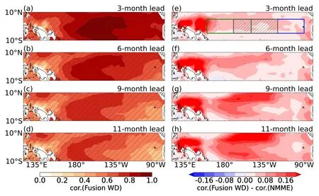
Fig.8.As in Fig.2 but for the prediction skill of the fusion model in which Wasserstein distance is used as the distance metric.

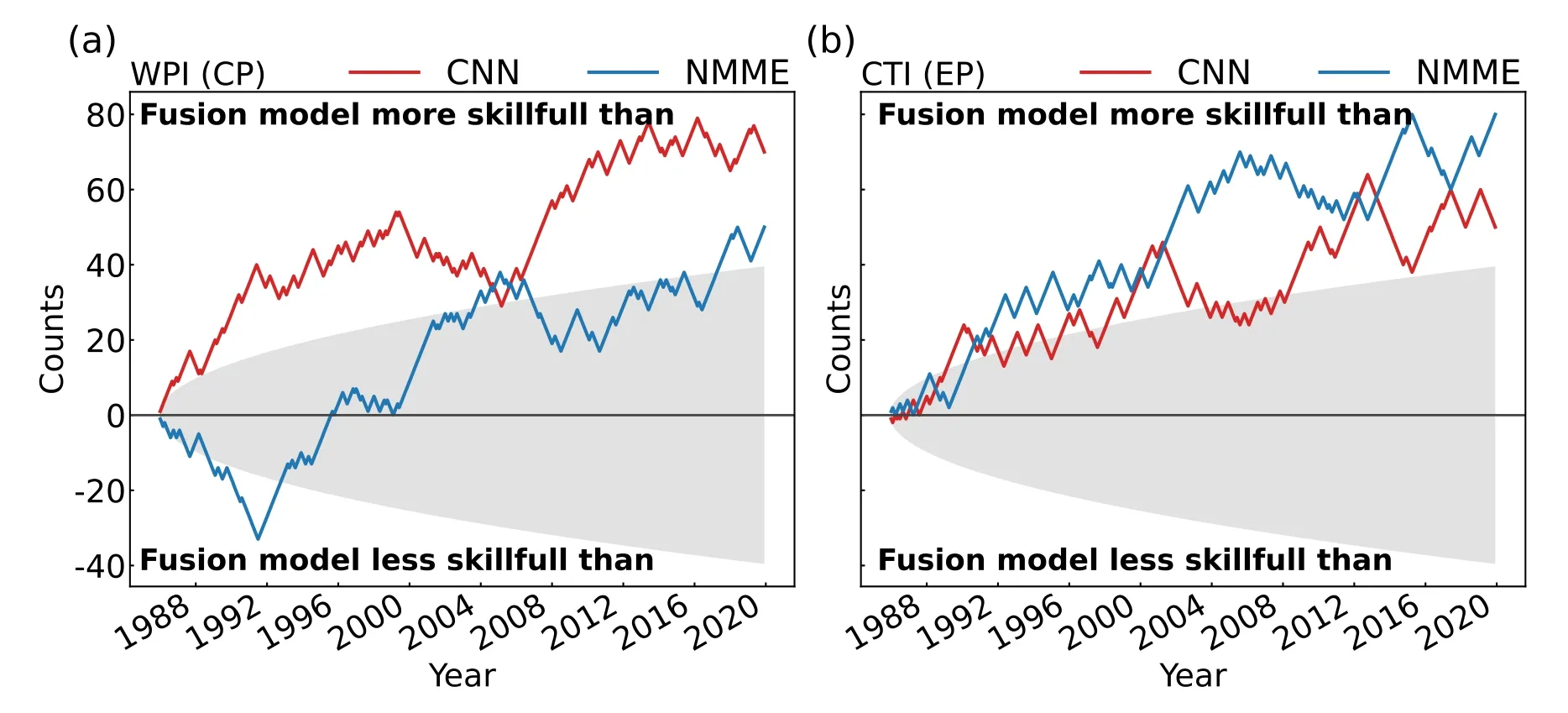
Fig.9.Prediction skill of the fusion model for (a) CP ENSO index and (b) EP ENSO compared with the CNN model and the NMME models at an 11-month lead time.The significance of the comparison is tested using the random walk method,and the shaded area represents the boundary of confidence at the 95% confidence level.

As shown in Fig.8 and Fig.S6 in the ESM,the fusion model as the CNN model possesses an apparent advantage relative to the dynamical models in the central Pacific,and the skill of the fusion model is comparable to that of the dynamical models in the eastern Pacific.As a result,the skill of the fusion model for both EP and CP ENSO is superior to that of the CNN model at lead times of three to eleven months,and each of the dynamical models except CanCM4i at lead times of seven to eleven months for EP ENSO.In particular,the skill for CP ENSO can exceed 0.7 at a lead time of up to ten months (Fig.3).Considering that the fusion model has only one member,we perform a significance test using the random walk method (Delsole and Tippett,2016).Figure 9 shows that the improvement in prediction skill of the fusion model with Wasserstein distance is significant compared with the CNN model and the NMME models.This result demonstrates that this new prediction strategy of fusing traditional dynamical models and a deep learning method is an effective way to improve ENSO prediction.

4.Discussion and conclusion

A deep learning model for predicting two-dimensional SSTAs in the tropical Pacific using a CNN model trained with CMIP6 simulations is constructed in this study.The predicted two-dimensional SSTAs clearly illustrate a superiority of the deep learning method in predicting the tropical Pacific SSTAs mainly located in the western and central equatorial Pacific.This superiority of the CNN model gives it a much higher prediction skill with respect to CP ENSO than dynamical models.The CNN model can distinguish the two types of ENSO at two-season leads,which has traditionally been a great challenge for dynamical models.An integrated gradients method provides a high level of interpretability for the CNN model,which is able to reveal the key precursors in the initial SSTAs to predict the different spatial modes of ENSO.The location-dependent superiority of the CNN model could be associated with the deep learning method being better at recognizing small-scale signals with larger influences in the western and central Pacific rather than the large-scale ocean dynamics dominating in the eastern Pacific.These results point out that the CNN model has potential limitations in predicting EP ENSO,and it has higher skill in predicting CP ENSO.

A recent study just using CMIP6 historical simulations to train a CNN model found that the prediction skill without transfer learning showed no considerable change in predicting ENSO (Shin et al.,2022).As there is no transfer learning applied in the present CNN model,the CNN model can be considered just as an extension of the outputs of the CMIP dynamical models.This result indicates that a nonlinear CNN method based on the outputs of CMIP dynamical models can greatly extend the ability of dynamical models in ENSO prediction.A fusion model combining the respective advantages of the CNN model and the direct prediction of dynamical models further improves the prediction skill for the two types of ENSO.The skill for CP and EP ENSO can exceed 0.7 at a lead time of up to nine and seven months,respectively,which is a marked improvement relative to the direct prediction of the dynamical models for the two types of ENSO.In this study,the superiority of the CNN model is discussed through comparison with dynamical models,but the differences between the CNN model and other empirical models for ENSO prediction are not yet clear,which should be explored in future.

To some extent,the attribution method reflects the advantage of the CNN model compared with the dynamical models in CP ENSO forecasting,which is expedient for the blackbox deep learning method.An event-based attribution method,the integrated gradients method,is chosen in this study for obtaining the heat maps.The integrated gradients method is selected as it can capture small-scale signals well,which is of importance for CP ENSO.There are also other attribution methods that can be used to derive heat maps,such as Class Activation Mapping (CAM),as used by Ham et al.(2019),and Grad-CAM,as used by Feng et al.(2022).The key difference from Grad-CAM is that the integrated gradients method calculates the features of the input data,allowing for the capture of smaller-scale signals.A comparison among different attribution methods is needed for improving the attribution of deep learning predictions in future studies.

Acknowledgements.The work was supported by the National Key R&D Program of China (Grant No.2019YFA0606703),the National Natural Science Foundation of China (Grant No.41975116),and the Youth Innovation Promotion Association of the Chinese Academy of Sciences (Grant No.Y202025).

Data availability.Data related to this paper can be downloaded from the CMIP6 database (https://esgf-node.llnl.gov/projects/cmip6/),NMME phase 1 (http://iridl.ldeo.columbia.edu/SOUR CES/.Models/.NMME/),and COBE-SST2 (https://psl.noaa.gov/data/gridded/data.cobe2.html).

Code availability.The codes for the CNN model can be obtained from the corresponding author.

Electronic supplementary material:Supplementary material is available in the online version of this article at https://doi.org/10.1007/s00376-023-3001-1.