Dynamic train dwell time forecasting: a hybrid approach to address the influence of passenger flow fluctuations
2023-11-18ZishuaiPangLiwenWangShengjieWangLiLiQiyuanPeng
Zishuai Pang · Liwen Wang · Shengjie Wang · Li Li,2 · Qiyuan Peng,2
Abstract Train timetables and operations are defined by the train running time in sections, dwell time at stations, and headways between trains.Accurate estimation of these factors is essential to decision-making for train delay reduction, train dispatching, and station capacity estimation.In the present study, we aim to propose a train dwell time model based on an averaging mechanism and dynamic updating to address the challenges in the train dwell time prediction problem (e.g., dynamics over time,heavy-tailed distribution of data, and spatiotemporal relationships of factors) for real-time train dispatching.The averaging mechanism in the present study is based on multiple state-of-the-art base predictors, enabling the proposed model to integrate the advantages of the base predictors in addressing the challenges in terms of data attributes and data distributions.Then,considering the influence of passenger flow on train dwell time, we use a dynamic updating method based on exponential smoothing to improve the performance of the proposed method by considering the real-time passenger amount fluctuations(e.g., passenger soars in peak hours or passenger plunges during regular periods).We conduct experiments with the train operation data and passenger flow data from the Chinese high-speed railway line.The results show that due to the advantages over the base predictors, the averaging mechanism can more accurately predict the dwell time at stations than its counterparts for different prediction horizons regarding predictive errors and variances.Further, the experimental results show that dynamic smoothing can significantly improve the accuracy of the proposed model during passenger amount changes, i.e.,15.4% and 15.5% corresponding to the mean absolute error and root mean square error, respectively.Based on the proposed predictor, a feature importance analysis shows that the planned dwell time and arrival delay are the two most important factors to dwell time.However, planned time has positive influences, whereas arrival delay has negative influences.
Keywords Train operations · Dwell time · Passenger flow · Averaging mechanism · Dynamic smoothing
1 Introduction
The train dwell time at stations is defined as the differences between the departure time and arrival time.Train dwell time, train running time, as well as train headway, are three crucial parts of railway timetables and train operations[1].Once any of the three parts is disturbed by unexpected factors (e.g., bad weather, infrastructure failure), train operations may be severely delayed, affecting the whole train operation process, or even the train operations on the whole railway network due to delay propagations [2].On the other hand, operators usually need to calculate the minimum needed train dwell time based on given parameters (e.g.,the number of station tracks, passenger flow, and technical operation times) to make the railway schedules in the timetable planning process [3].Also, railway station capacity calculations require the train dwell time to be known.Therefore, accurate estimation of train dwell time is of great importance to decision-making during train delays, timetable planning, and station capacity estimation [4].
However, train dwell time is potentially influenced by complex factors (e.g., train delays due to interruptions, timetable structure, and passenger flow) [5, 6], which considerably lowers the predictability of train dwell time [7, 8].For example, train dwell time is affected by delays.When trains are delayed, the traffic controllers tend to use the recovery time pre-scheduled in railway sections or stations to reduce the train delays [5].This means the train dwell time can be shorter than the planned when the trains are delayed.Further, trains of different speeds, service lengths/durations, and categories (e.g., freight or passenger trains, or long-distance trains and regional trains), usually run on the same railway line/infrastructure [9].One of the main functions of the train dwell process is the overtaking of different train services.Trains that are overtaken by other trains inevitably have longer dwell time due to the minimum headway requirement of train operations.Finally, another primary purpose of train dwell is to serve passengers (i.e., passenger boarding and alighting), which means that the number of boarding and alighting passengers noticeably influences the train dwell time, especially on peak hours, weekends, and public holidays.Therefore, accurate prediction of the train dwell time requires advanced tools that take the complicated factors (influencing factors, data characteristics) into account.
Existing train dwell time models usually use a single predictor to estimate the train dwell time [10].This inevitably makes the prediction model unable to address the complicated influencing factors [11].Further, traditional train dwell time models failed to consider the real-time passenger amount.However, the passenger soars and plunges in different periods distinctively influence the train dwell time.We propose a hybrid train dwell time prediction model for real-time train dispatching based on an averaging mechanism and dynamic updating to address these problems.The averaging mechanism is based on multiple state-of-the-art base predictors, enabling the prediction model to integrate the advantages of different base predictors.Dynamic updating uses real-time passenger flow data to update the predicted results of the model,making the prediction model take the real-time passenger changes/fluctuations into account.Through the usage of an averaging mechanism based on multiple predictors to predict the train dwell time the model thus can address more complicated problems in terms of data types and distributions,in comparison to the existing dwell time prediction models based on a single predictor.The proposal of the updating mechanism improves the capacity of the model in addressing the passenger soars or plunges during different periods.In addition, we have combined the train operation and real-time passenger data for dwell time prediction.
The remainder of this study is structured as follows.In Sect.2, the existing studies about vehicle dwell time estimation are reviewed, and the problems in train dwell time prediction are discussed.In Sect.3, the data information used in the study are provided, and the influence factors are determined.In Sect.4, we introduce the proposed model.Finally, the experimental results are presented in Sect.5.
2 Related work and problem statement
2.1 Related work
Recent review studies in the field of railway transport show that predictions mainly lie in train delay prediction,running time modeling, and dwell time modeling [12-14].Train delay prediction has been studied deeply; examples include graph-based models [15], machine learning models[16], and hybrid models [17].Train running time has been mainly modeled from a probabilistic perspective.For example, probability distributions were used to interpret the train running time, on which train arrival time can be estimated [18].Besides, train operation conflict detection and conflict resolution [19] and control actions prediction[20] are typical ways to train operation modeling.
Dwell time estimations are critical for real-time traffic management of passenger assignments [21].Generally, the dwell is mainly influenced by two factors,i.e., the passenger flow (e.g., the boarding and alighting passengers) and the delays of the vehicles.Due to the complicated relationships between the factors and vehicle dwell time, many state-of-the-art methods have been proposed to estimate dwell time from different perspectives.The main focuses lie in estimating bus and train dwell time at stations.The proposed methods include statistical, probability, machine learning, and hybrid models.
According to an investigation, the most critical factors for bus dwell time prediction include passenger activity, lift operations, and other effects, such as low-floor bus, time of day, and route type [22].A recent investigation on train dwell time with the operation and passenger flow data shows that the passenger amount at the critical door is the most influential variable for a late-arrival train.In contrast, the scheduled dwell time and the deviation from the scheduled arrival time are the essential variables for early trains [23].Different data from diverse systems have been collected to achieve different purposes or study the problem from different perspectives to predict the bus dwell time at stations.Typical examples include using automatic vehicle location systems[24, 25], global positioning systems [26], and automatic passenger counters systems [27], to record the data on which the dwell time or travel time models were established.The proposed bus dwell time prediction models include log-linear and quantile regression [28], gene expression programming[29], and stochastic models [30].In addition, Padmanaban et al.[31] incorporated the bus stop delays associated with the total travel times of the buses under heterogeneous traffic conditions to build a reliable algorithm that can be adopted for bus arrival time prediction under Indian conditions.Meng et al.[30] first pointed out that due to the merging behavior of buses and vehicles on the shoulder lane, the dwell time of buses at bus stops is highly uncertain.The authors developed a new probabilistic method to estimate bus dwell time, including a standard regenerative stochastic process to simulate the interaction between bus, arriving passengers, and shoulder lane traffic.A specific method is also proposed to estimate the average value and random bus dwell time variables.Li et al.[32] built a linear model and a nonlinear model to estimate the bus dwell time in the rapid bus systems.The conflicts between passengers boarding and alighting were integrated into the prediction models.This model thus showed outperformance over the proposed model in Ref.[27].
Different from the bus dwell time that is mainly influenced by vehicle states and passenger flow, train dwell time (i.e., metros or railways) is also highly dependent on the planned dwell time, as the train operations on rail tracks need to synchronize with each other [15].This is mainly because the departure time of railways is published to the passengers.Therefore, the trains cannot depart at stations earlier than their planned departure time.This means that the actual dwell time of trains is influenced by passengers,vehicle types/states, and timetable parameters [13].In addition, supplement time is usually set at sections or stations to absorb train delays.The minimum train dwell time can usually be determined from historical operation data.For example, one can investigate the minimum dwell time in each period for each station by statistics or technical files.A recent review study [10] indicates that the proposed prediction models for train dwell time at stations include statistical models (e.g., distribution models [33-35],regression model [36-38]), simulation models (e.g.,microscopic model and macroscopic model [39-41]), and other models (e.g., fuzzy logic [42, 43], extreme learning model [44], random forest [5], and hybrid models [45-47]).D’Acierno et al.[48] innovatively proposed a dwell time estimation model based on the crowding level at platforms and related interaction between passengers and the rail service.A case study based on metro systems showed the feasibility of the method.In addition, Cornet et al.[49] proposed to split the dwell time into a deterministic component that depends on the passenger flow, called the minimum dwell time, and a random component that depends on the system states (e.g., interruptions and delays).Then,they developed a method to estimate the two components respectively.Buchmüller et al.[50] developed a calculation method for train dwell time at stations for timetable planning based on automatic passenger counting systems.A summary of the train dwell time model demonstrates that using the passenger flow (i.e., the number of boarding and alighting passengers) to estimate the train dwell time is appropriate.However, there is a lack of further explorations of train dwell time to improve the punctuality of trains [50].Further, the authors of Ref.[51] have proven that boarding and alighting passengers have noticeable effects on train dwell time.They reviewed the studies that used regression coefficients to describe passenger alighting and boarding times.They concluded that the alighting time ranges from 0.4 to 1.4 s per passenger, whereas the boarding time ranges from 1.4 to 2.4 s per passenger.
A summary of the train dwell time model is shown in Table 1.The reviewed study shows that regression models have proved to be a valuable tool to describe observed data and test the relationship between residence time (i.e.,independent variable) and corresponding factors (dependent variable) [10].Specific rules and assumptions need to be established in advance for the simulation model.The model’s accuracy largely depends on the selected parameters and basic conditions.Hybrid and innovative methods may take residence time modeling to a new stage.Therefore, we propose a hybrid model based on an averaging mechanism to overcome the weaknesses of a single predictor on the complex data, and use a dynamic updating system to update the predictive results of the averaging method.The model takes the train operation and passenger boarding and alighting information into account, aiming at improving train operation management and control.

Table 1 A summary of train dwell time estimation models
2.2 Problem statement
Train operations are influenced by unexpected factors inside or outside the systems.Specifically, the train dwell process at stations is for passenger boarding and alighting, train overtaking, and technical inspections.The train overtaking and technical inspections are standard, meaning that the required time cost of these two processes is primarily constant in a railway system.However, passenger flow exhibits spatialtemporal differences.For example, at the main station of the railway lines or during peak hours, the passenger flow is usually much more than passenger flow at the standard stations and off-peak hours.Figure 1a, b shows the distribution of actual dwell times of trains at the stations over the time of day and stations in the Wuhan-Guangzhou high-speed railway line in China (the acronyms of stations in Fig.1b are explained in Fig.2).It clearly indicates that the actual train dwell time is diverse in time and space.This is understandable, as the passenger flow shows spatiotemporal differences.Most importantly, extreme passenger flow (e.g., on public holidays) will considerably influence the dwell times of trains at stations, making the traditional prediction model incapable of predicting the dwell time under these situations.
In addition, train operations are composed of running processes in sections and dwell processes at stations.The continuous quality of train operations means that any past train operation patterns quickly propagate to the future.For example, Fig.1c shows the train operations during a disruption.To avoid conflicts, trains operating during the disruption were slowed down, meaning that the train running time was longer than the planned.Due to the influence of the disruption, the train may also dwell longer than the planned.This means that the train dwell time may be longer than the planned when the train running time was longer than the planned for the previous section.Therefore, train dwell time prediction needs to allow for train operation-related parameters in the previous sections and stations.
In summary, the analyses above clearly show that the actual train dwell time is influenced by the passenger flow and the past train operation-related processes/states.The previous studies only used a single predictor, e.g., regression model [36], and random forest [5], to predict the train dwell time.However, the diverse types of influence factors make the predictor's performance unstable (a common drawback of the machine learning model on the complex dataset).In addition, these models were all trained on common passenger data and train operation data, making them incapable of predicting the sudden increases/decreases in dwell times under extreme situations (e.g., on public holidays).
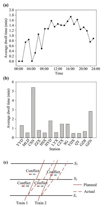
Fig.1 Actual dwell time distribution over a time and b space, and c train operations during conflicts
To improve the robustness and predictive performance of the prediction model, an advanced predictor is needed to cope with the diverse data types and extreme situations.Therefore, to overcome the drawback of a single predictor in addressing the diverse data types, we propose a hybrid method based on an averaging mechanism to predict the train dwell time for real-time train dispatching.The proposed model is expected to integrate the advantages of different machine learning models, thus improving the robustness and predictive performance of the model.Further, the proposed model uses a smoothing technique to update the model predictions under extreme situations(e.g., on public holidays).These qualities of the proposed model enable it to predict the train dwell time more accurately under any situation.
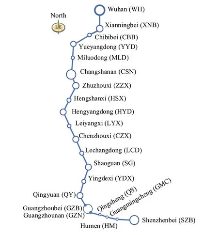
Fig.2 The layout of the WH-GZ HSR
3 Data and influence factors
3.1 Data description
The data used in this study comes from one of the busiest and the most early-open high-speed railway lines, i.e.,the Wuhan-Guangzhou line (WH-GZ HSR).The layout of this line is shown in Fig.2.This line includes 16 stations in total, where this study focuses on the train operations at 14 stations and 13 sections, i.e., from Yueyangdong station to Guangzhounan station, approximately 1000 km.The data include the train operation records for one year,from December 2015 to November 2016.In this period, the number of daily average train services was 118 in a single direction.The train operation speed on the WH-GZ HSR in this period is 300 km/h, whereas trains can be speeded up to 310 km/h when they are delayed.The train operation data contains the planned/actual arrival and departure times of each train at each station, with a unit of a minute.Table 2 demonstrates a few cases of train operation observations.

Table 2 Examples of train operation data

Table 3 The passenger flow data
Passenger flow data were also used to accurately predict train dwell time at stations.The passenger flow data include the number of passengers between each pair of stations,i.e., the origin and destination (OD) pairs.Table 3 shows a fragment of the passenger flow data of train G1006 on 2nd December 2015.Based on the passenger flow data in Table 3, we thus can calculate the number of boarding and alighting passengers in each train at each station.
3.2 Influence factor investigation
With the data introduced above and domain knowledge (e.g.,the technical requirements of train operations), the potential influence factors of the train dwell time at stations can be determined.Since one of the main objectives of the train dwell process is to serve passengers, the number of boarding and alighting passengers will affect the train dwell time at stations.Generally, the more passengers are served, the more dwell time tends to be.To demonstrate the influences of passengers on train dwell time, we fit a multiple linear regression model by treating the number of boarding passengers (MBP) and the number of alighting passengers(MAP) of each train and station as independent variables, and the actual train dwell (TW) times in stations as the dependent variable.The final fitted linear model is shown as
The fitted linear model in Eq.(1) clearly shows that the coefficients of the number of boarding and alighting passengers are similar (equaling 0.010 and 0.011,respectively), indicating that they have almost equivalent impacts on the actual train dwell time.In addition, this equation indicates that serving 100 more passengers will approximately lengthen dwell time of 1 min at the station.Overall, these results show that the number of passengers notably influences the train dwell time, and quantitatively demonstrate the relationships between dwell time and passenger volume.
The reason why we use a regression model is that it can show the influence of passenger demand on dwell time quantitatively.For example, how long the dwell time will be prolonged due to one more boarding and alighting passenger? However, a machine learning model usually addresses the relationship between the input (boarding and alighting passengers) and output (i.e., dwell time) as a black box.Therefore, we do not use a machine learning model because it cannot quantitatively show the coefficients of boarding and alighting passengers on dwell times.
Railway trains are expected to operate on schedule.The planned train dwell time needs to meet the passenger boarding and alighting requirements.A large number of passengers usually mean long-planned train dwell time.Based on this train operation requirement, the planned train dwell time at the station intuitively influence the actual train dwell time.
Then, train operations are continuous, meaning that any pattern (e.g., slowing down and speeding up) may propagate to the near future.This means that the near past information can influence the dwell time at the station.A typical example could be when trains operate during disruptions, the delay will be continuously increasing.This means that if the train spends more time (than the planned one) in the previous section, it is likely to spend more time at the current station due to the influence of disruptions.Next, if a train is delayed,the traffic controllers may recover the train delay by reducing the dwell time in stations (but the train departures cannot be earlier than the planned one to serve the passengers).Therefore, we select the near past train operation-related processes and states as the input of the dwell time prediction model, including the actual and planned running time over the previous section and arrival delay of the train at the to-be-predicted station.
Finally, other than serving passengers, another objective of train dwelling at the station is to be overtaken by other trains.If a train is overtaken by other trains, its dwell time tends to be longer than the one without being overtaken, due to the minimum headway requirement between consecutive trains.Therefore, we also defined a binary variable (1 denotes the train will be overtaken by other trains, and 0 denotes the otherwise) in the input of the model to contain the overtaking information of trains.
Based on the train operation data, passenger flow data,and the variables determined above, the values of each variable can be extracted.The observations that were extracted from the data contain 785 cases.Table 4 lists six cases (a fragment) of the data for train dwell time prediction,whereas the calculations of these variables are shown in Eqs.(2)-(5).To avoid over-fitting, we randomly split the data into training data (accounting for 70%, 549 cases) and testing data (accounting for 30%, 236 cases).

Table 4 Final data for train dwell time prediction based on the influence factors investigation
4 Method
In this section, we first introduce the structure of the proposed model; then, the base predictors for the averaging mechanism are introduced, and the experiments for determining the hyper-parameters of the base predictors are designed.
4.1 The proposed model
Machine learning (ML) and deep learning (DL) models usually show different advantages in addressing problems.For example, the decision tree-based models (e.g., random forest) are robust to unbalanced data [51]; neural networks are robust to factors with different importance to the target, as the weights of the neurons can be trained to (close to) zero if a factor has insignificant impact on the target; further, the convolutional neural networks have been used in railway systems to capture the spatiotemporal dependencies for predicting train delays; thek-nearest-neighbors (KNN) model is insensitive to outliers, as it just selectsknearest observations to update the algorithm.However, transportation systems are complex and involve multiple sub-sections/sub-systems.Typically, railway systems are influenced by complex factors (e.g., passenger flow, operators, and timetables).These factors basically show different characteristics (e.g., data distributions, feature importance, and data attributes).This means that the predictive model in the railway systems based on a single predictor is easily affected by the complex data attributes.In addition, transport services are easily delayed because of the significant increase in passenger flow [10,40].However, standard machine learning models trained on normal passenger data cannot capture real-time passenger increases.To improve the robustness and performance of the proposed model, we use the averaging mechanism to address the disadvantages of a single ML model, and a dynamical updating mechanism to address the problem that standard ML models cannot capture the real-time passenger soar or plunge.The structure of the proposed model is shown in Fig.3.
In the proposed model, we first used four state-ofthe-art ML models, i.e., the gradient boosting decision tree (GBDT), random forest (RF), KNN, and convolutional neural networks (CNN) to predict the train dwell time in normal situations.The GBDT and RF models are both tree-based; they show superior performance on unbalanced data.The CNN model can address the various dependencies between input and output variables by updating the neuron weights; further, the CNN is able to learn the dependencies between the input factors, as its convolutional filters parallely operate on multiple input features.Finally, the KNN model can better address the outliers.Thus, the proposed hybrid model is expected to perform better, as it integrates the advantages of the four base predictors.Here, to obtain the final predictive results,an unweighted averaging is performed over the four base predictors.We combinedly trained them and tuned their parameters.A fivefold cross-validation technique based on a grid-search method was used in the parameter tuning process.Then, the final result of the proposed model is the average of the four base predictors.In other words,we use the mean values of the four base predictors as the prediction of the proposed method.This enables it to outperform other base methods regarding predictive errors and variances.
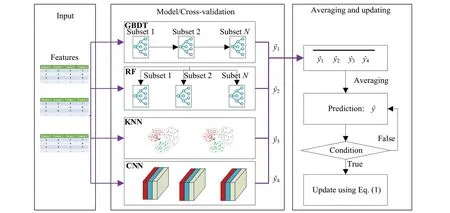
Fig.3 Framework of the proposed method based on the averaging mechanism
The machine learning method only predicts the dwell time based on the train operation data and passenger amount.However, they cannot address the situations when the passenger flow soars (e.g., on weekends and public holidays).To address this problem, we use a dynamic updating mechanism that considers the real-time passenger flow information (based on the passenger flow regression coefficients in Eq.(1)), to update the final prediction of the machine learning models, as shown in the final step/block of the model in Fig.3.Here, the condition performing the updating is: if the dwell time calculated with Eq.(1) is longer than the planned dwell times.In real-time train dwell prediction, the operators can also judge if the condition is met using the real-time passenger flow and Eq.(1).This enables the proposed model to address the real-time passenger soar, thus making it suitable in any situation.
4.2 Base predictors
In this section, we briefly introduce the four base predictors we used in the proposed model, namely CNN, GBDT, RF,and KNN.
4.2.1 Convolutional neural networks (CNN)
The two-dimensional CNN is a neural network model that is widely used in image recognition and data discovery[52].Its main advantage over the standard neural networks (i.e., multilayer perceptron, MLP for short) lies in its convolutional filters/kernels, which operate on multiple local elements (i.e., pixels for images), in comparison to MLP that each neuron only operates on a single element.This quality of the CNN model enables it to capture the dependencies within the local elements [52].The difference between the one-dimensional CNN (1D-CNN) and two-dimensional CNN (2D-CNN) is that the convolution kernel of the 2D-CNN applied to the inputs is twodimensional, while the convolution kernel of the 1D-CNN applied to the time series is one-dimensional, as shown in Fig.4.
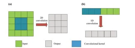
Fig.4 Schematic diagram of the artificial neural network: a 2D-CNN; b 1D-CNN
The CNN model is also a mathematical α mapping of the input features.Given the input features,xk∈RK, whereKis the number of features, and the label,ym∈RM, whereMis the number of categories.The CNN model first applies the filters/convolutional kennelWkon the input, and then is activated by a nonlinear functionσ(X) on the convolutional result and the bias:
wherehkis the output,Xis the input,Wkis the convolutional filter/kernel,bis the bias of the layer, andσis the activation function.
4.2.2 Gradient boosting (GB)
The GBDT [53] is a combination of the boosting technique[54] and classification and regression trees (CARTs).The boosting technique trains a weak classifier (CART in GBDT)with initial weights from the training samples first, and then updates the weights of samples according to the learning error rate of the weak classifier.If the weights of the training samples with significant learning error rates in the weak learner, they will be adjusted to be more significant after training.Then subsequent weak classifier will pay more attention to these samples with high error rates and use the adjusted weight in the previous classifier to train the current weak classifier.This process is repeated until reaching the specified number ofTweak classifiers.In other words,boosting means training a bunch of models sequentially.Each model learns from the mistakes of the previous model.Finally, theseTweak classifiers are integrated to obtain the final strong learner.
The GBDT generates a weak classifier in each iteration.Assume the weak classifier and loss function in the previous iteration areft-1(x) andL(y,ft-1(x)) , respectively.The target of this iteration is to establish a CART,ht(x) , which can minimize the loss in this iteration (i.e.,L(y,ft(x))=L(y,ft-1(x))+ht(x)).The negative gradient of loss functionLis used to fit the approximate value of loss function in this iteration, resulting in establishing a CART,in which the negative gradient of the loss function of theith sample in thetth iteration is presented as
whereθis the intercept.Accordingly, the CARTht(x) can be presented as
The final classifier is obtained given different weights of the weak classifiers in each iteration.
4.2.3 Random forest (RF)
The perspective of RF is to build a forest randomly with many CARTs [55], while there is no correlation between each decision tree in the random forest.For each tree, the bootstrap sampling technique [56] is used.Given a datasetDmwithmsamples, in the bootstrap sampling technique,each sample in the training dataset will be selected fromrandomly and then returned to theDM(i.e., the sample may still be sampled in the subsequent sampling).After executingmtimes, a dataset containingmsamples is the sampling result.Relying on the bootstrap sampling technique, several training datasets(assuming it isN) are obtained by repetitive and independent sampling.Kfeatures from each training dataset (Kis less than the full features of the original data) are chosen randomly and inputted into a CART for each training dataset.Once a new sample is inputted, each decision tree in the forest votes to decide which category the sample should belong to.Overall, the RF uses the bagging technique, which is performed in a parallel combination of decision trees, in comparison to the boosting, which is performed sequentially.Each model learns from the mistakes of the previous model.According to the vote results of all trees, the most selected category is the sample category for the classification task, while the average value of all trees is the output for the regression task.The structure of the random forest is shown in Fig.5.

Fig.5 RF structure
4.2.4k-nearest-neighbors (KNN)
The algorithm idea of KNN is to find thekmost similar data in the given dataset to determine the category of prediction data.The KNN has no loss function, while there are three critical parameters for KNN to determine the prediction performance.The first one is the number of neighbors (i.e., the value ofk).Generally, a small value is chosen to be the initial value according to the sample distribution, and then a more appropriate value will be updated through cross-validation.The second parameter is how to measure the distance between data.Some commonly used distance methods (e.g., Euclidean distance in Eq.(11)) can be used to measure the similarity.
4.3 The exponential smoothing
The exponential smoothing method is a particularly weighted moving average method.The function of the exponential smoothing method is to strengthen the impacts of recent observations on the predicted values.The weights given to observations at different times are diverse, thus increasing the weights of recent observations.Therefore,the predicted value can quickly reflect the actual changes in the real world.The weights are reduced by an equal ratio series, the first term of which is the smoothing constanta,and the common ratio is (1 -a).Second, the exponential smoothing method is flexible to the weights given by the observed values, and different values can be taken to change the rate of weights.Ifais taken as the smaller value, the weight changes more rapidly, and the recent change trend of the observed values can be reflected in the moving average of the index more quickly.Therefore, different values can be selected using the exponential smoothing method to adjust the uniformity of the observed values of the time series (i.e.,the stability of the trend change).
wherestis the smoothed statistic,xtis the observations at the current time step, andst-1is the previous smoothed statistic(at time stept-1).Here, to capture the real-time passenger information, we treat the values obtained based on Eq.(1)as the observations at the current timestep, and the predicted values of the averaging mechanism (based on the four ML models) as the statistic at the previous step.
We use the procedure in Fig.6, when applying the smoothing technique to the predicted values of the proposed model.The critical step is the judge the passenger amount.In the present study, if the dwell time calculated by Eq.(1) is longer than the planned dwell times, the smoothing technique will be applied.For instance, if both the real-time boarding and alighting passengers are 100, the dwell time calculated by Eq.(1) should be 3.902 min; if the planned dwell time is 3 min(3.902 min > 3 min), the smoothing will be used to update the model.It should be noted that the real-time passenger amount can be calculated based on the ticket-selling system.
4.4 Experiments for parameters
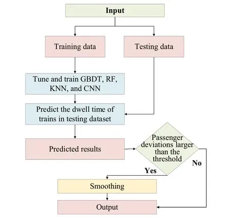
Fig.6 An outline of using the smoothing in the proposed model
The proposed prediction model contains four base predictors, the GBDT, RF, KNN, and CNN.Each model has different hyper-parameters.In this section, we experimented to tune one of the most important parameters of each model.The GBDT and RF are composed of decision trees, and the final outputs are the averages of the averaging results of each decision tree.Therefore, the number of estimators/decision trees is one of the most sensitive hyper-parameters to the performance of the prediction model.The candidate for the number of estimators of the GBDT and RF model include [50, 100, 150, 200].The KNN model performs classification or regression based on the features/characteristics ofkneighbors, meaning that the hyper-parameterkis sensitive to the performance of the model.The candidates for the hyper-parameterkinclude [2, 3, 4, 5, 6, 7, 8].Finally, the CNN model is composed of neural network layers, where each layer contains a different number of filters.Therefore, we experimented with the structure of the CNN (including different matches of layers and neurons).The candidate CNN structures include [(32, 32, 32), (32, 64), (96,)].Here, for the CNN, we use 96 neurons, which can be distributed into a different number of layers.The length of tuples represents the number of layers, and the values represent the number of neurons in each layer.For example, the tuple (32, 64)means that the CNN has two layers, the first with 32 and the second with 64 filters.
We use a grid-search method based on fivefold crossvalidation to tune the abovementioned hyper-parameters.Here, the parameter tuning and cross-validation are performed using the training dataset.To avoid over-fitting,we separate the training data into two parts, 80% is used to train the model, and the remaining is used to demonstrate the performance of the model.The search results are evaluated based on the goodness of fit,R2, as shown in Eq.(13).TheR2over the combinations of different hyper-parameters is shown in Fig.7.Based on the gridsearch results, we thus can select the hyper-parameters that resulted in the highestR2as the hyper-parameters of the proposed model, i.e., the number of estimators for GBDT and RF is 50 and 100, respectively; the parameterkfor KNN is 2; and the CNN structure is (32, 64).The optimal hyper-parameters are shown by the black line in Fig.7.
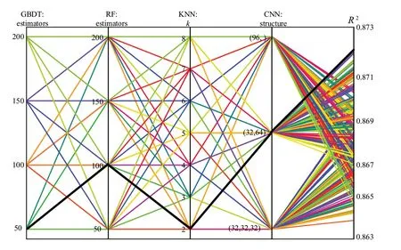
Fig.7 Grid-search results of hyper-parameters based on cross-validation
whereNis the number of samples,oiis the observed value,piis the predicted value, andis the mean value of observations.
5 Results
In this section, we first evaluate the performance of the proposed model based on the testing dataset.Then, the importance of the influencing factors is shown by sensitivity analysis.
5.1 Predictive result analysis
To show the performance of the proposed model, we first demonstrate the predicted values and the residuals.The box plot in Fig.8a shows the comparison between the predicted values and the actual dwell time, where the main body of the box (the lower whisker to the upper whisker) shows the distribution of the dataset, and the points above the main body are detected as outliers.This figure clearly shows that the main body of the actual and predicted dwell time are similar, indicating the high accuracy of the predictive model.We also show the residual (the difference between the actual and predicted dwell time) in Fig.8b.In this figure, the horizontal axis represents the number of observations, and the vertical axis represents the corresponding residual of the cases.The result shows that the residuals of the prediction model are all-around zero, indicating the effectiveness of the predictor.In addition, the mean line (red) is located at zero,indicating that the residuals satisfy the zero-mean assumption of regression models.
5.2 Evaluation of the averaging mechanism
In this study, an averaging mechanism is used to improve the robustness of the dwell time prediction model.The averaging mechanism is based on four base predictors, namely GBDT,RF, KNN, and CNN.The averaging method is expected to integrate the advantages of the four models in addressing different data problems.To evaluate the performance of the averaging method, we select these four base predictors as the benchmark model to quantitatively show the improvements of the averaging method.The introduction of these four base predictors can be seen in Sect.4.2.
We used four other standard regression model evaluation metrics, namely mean absolute error (MAE), root mean squared error (RMSE), mean absolute percentage error(MAPE), andRsquared (R2), to show the comparative results.The calculations of these metrics are shown in Eqs.(13)-(16).It should be noted that we chose different metrics because the MAE is a better metric for normal data; the RMSE can better demonstrate the performance of the model on outliers; the MAPE is to measure the relative errors; andR2is to demonstrate the goodness-of-fit.Additionally, the predictive variance is also a direction to evaluate the performance of a predictive model.A model with lower variances (more certain results) can provide more accurate predictions.Reducing the variance in dwell time is essential for the provision of information to travelers [14].In the present study, we used the standard deviations of the absolute errors to show the performance of the model on predictive variances.The standard deviation can show the sparsity of the predicted results.

Fig.8 Predictive results: a comparison between the actual and predicted values; b the distribution of residuals
To systematically evaluate the model, we show the performance of the proposed model (averaging) and the benchmark model on the cases from each railway station on the WH-GZ HSR and the cases on the HSR line combined.The comparative results of the different models in terms of MAE, RMSE, and MAPE are shown in Tables 5 and 6.The results in Tables 5, 6 clearly show that the proposed averaging method has lower errors than other benchmark models.
Additionally, the goodness-of-fit (represented byR2) of the predictive model to the testing data is shown in Table 6.This table shows that the predictors have distinctive goodness-of-fit to stations.The results show that theR2can reach 0.97 at YDX, and it can be as low as 0.05 at HSX.This is probably because the average dwell time differ from stations.Overall, theR2of the proposed model is 0.906, the highest among all the methods.This indicates the better performance of the proposed model.
Finally, the predictive variances (standard deviations),shown in Table 7, also indicate that the proposed model outperforms other models.These results further show the significance of using the averaging mechanism to improve the robustness and performance of the dwell time prediction model.

Table 5 Comparative results of different models in terms of MAE and RMSE (unit: min)
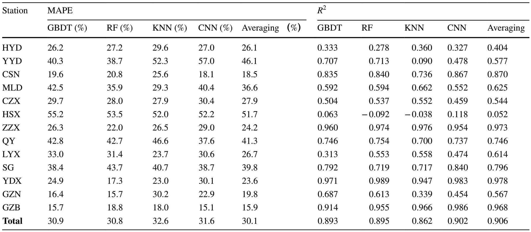
Table 6 Comparative results of different models in terms of MAPE and R2
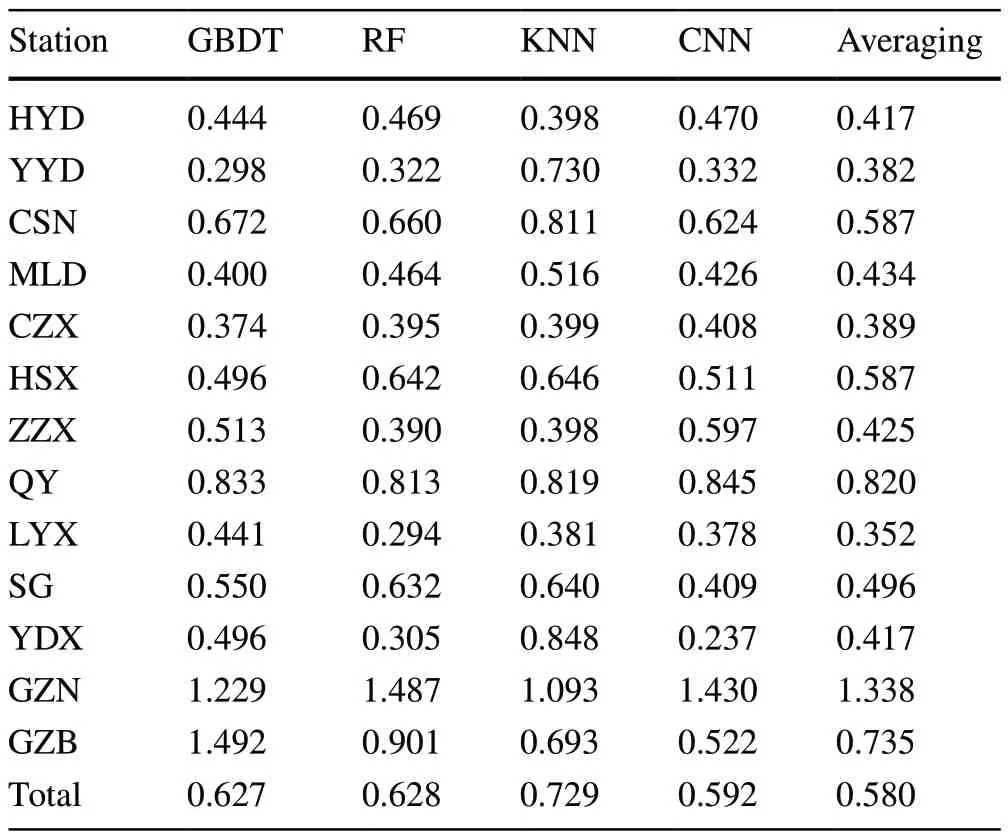
Table 7 Comparative results of the proposed model and the base predictors in terms of standard deviations of absolute errors
To show the advantages of the proposed averaging method across the four predictors, we compare it against other combined models.Here, because the GBDT, RF, and CNN models show better results among the four base predictors, shown in Tables 5, 6 and 7, we select the combinations of any two models as the baseline.For example,“GBDT + RF” in Table 8 represents the averaging result based on the GBDT and RF base predictors.
From Table 8, we can view that the proposed averaging method (i.e., averaging across the four predictors)outperforms other combined models (i.e., averaging across any two models among GBDT, RF, and CNN).This result is understandable, as the proposed averaging is performed on four predictors; the proposed averaging method is, thus,more robust to data; this also supports our assumption that each base predictor has its advantages in addressing data;for instance, GBDT and RF have better performances on the less-frequent samples; CNN has better performance on the samples whose features have inner dependencies; the KNN is insensitive to outliers.Further, the result in Table 8 can also be inferred from the results in Tables 5, 6 and 7, where they show that the proposed averaging outperforms all other base predictors.
5.3 Performance on long horizons
The proposed model predicts the train dwell time based on the arrival delay and running time in the previous section.This, to some extent, harms the applicability of the model in real-time train traffic control, as the model can only be performed when trains arrive at the station (where the dwell time needs to be predicted).To improve the applicability of the model in real-time train traffic control, we investigate its performance on longer horizons (i.e., one-station, twostation, and three-station in advance).
We also used the evaluation metrics introduced in Eqs.(14)-(17) to show the comparative results.Figure 9 shows the predictive errors of the proposed method and the base predictors on the testing dataset for one-station,two-station, three-station, and four-station prediction.It should be noted that the four-station prediction horizon(time ahead) can reach approximately 1 h, as the average running time between stations on the W-G line is 15 min.From Fig.9, we can conclude that: (1) the performance of the proposed method is superior to that of the base predictors; (2) with the increase of the prediction horizon,the predictive errors increase; and (3) the errors increase sharply first (from one-station to two-station predictions),and increase slowly when the prediction horizon is longer than two stations.

Table 8 Comparative results of models averaging across different base predictors (unit: min)

Fig.9 Comparative results of models on long-horizon prediction: a MAE; b RMSE; c MAPE; d R2
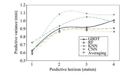
Fig.10 Comparison of model predictive variance
In addition, Fig.10 shows the comparative results of the predictive variance (represented by the standard deviation of the absolute errors).It also shows that the predictive variance increases considerably at first; then, the curves become stable and slow from the two-station horizon.The increase in predictive variances can be interpreted by the model uncertainty and data uncertainty, which is shown to exist in predictive models and training data.

Fig.11 Comparison between the actual and predicted dwell time
5.4 Dynamic updating using real-time passenger flow
The previous sections (Sect.5.1 and 5.2) have shown that the proposed prediction model based on averaging exhibits small predictive errors, and outperforms its counterparts(the benchmark models).However, real-time train dispatching, which the dwell time prediction model contributes to,needs real-time passenger flow information.As mentioned in Sect.2.2, the passenger soar easily influences train dwell time, leading to unpredictability in the standard ML models.This can also be ascertained from the comparison between the predicted values and actual values in Fig.8, where the solid red line represents the perfect predictions, i.e., the predicted values equaling the observations.Figure 11 clearly shows that the proposed model can accurately predict the short dwell time (e.g., not longer than 8 min), as the black points evenly distribute around the solid red line.However,the model tends to underpredict the long train dwell time(e.g., longer than 10 min), as these points distribute under the solid red line.This can also be ascertained from Fig.8a,where the bottom edge of the box of the predicted dwell time is slightly lower than that of the actual dwell time.This is mainly because the proposed ML model underpredicts the actual train dwell time under the condition that the passenger flow considerably increases.In other words, the unpredictability of these points is due to the influence of passenger flow.
To address this problem, we perform the last step of the proposed method in Fig.3, i.e., the smoothing/updating.The first step of performing the smoothing technique is to determine the parameterain Eq.(12).Here, this parameter was determined based on the confidence of the two variables, i.e., the predicted dwell time based on Eq.(1) and the predicted dwell time based on the proposed predictive method.The calculation of the parameter is shown below:
whereσpis the standard deviation of the predicted dwell time based on Eq.(1), andσvis the standard deviation of the predicted dwell time based on the averaging/proposed method.
We treat the values predicted based on Eq.(1) as the observations at the current timestep, i.e.,xtin Eq.(12), and the predicted values of the averaging mechanism (based on the four ML models) as the statistic at the previous step,i.e.,st-1in Eq.(12).Based on Eq.(17), the parameterain the study is 0.737, meaning the final predictions pay more attention to the recent information (i.e., the real-time passenger flow).We select the cases by considering the criteria in Fig.6 to test the performance of the smoothing technique.The cases are split into two groups, i.e., the number of total passengers in [min, 300), and the number of total passengers in [300, max].The metrics MAE and RMSE were used to demonstrate the performance of the averaging and “averaging + smoothing” methods, as shown in Fig.12.This figure clearly shows that smoothing can noticeably improve the performance of the predictive model, indicating the significance of using real-time passenger information.The results show that the smoothing can, on average, improve the performance of the prediction model by 15.4% and 15.5%, in terms of MAE and RMSE, respectively.
5.5 Feature importance analysis
Identifying the most important features to dwell time is critical for traffic operators and controllers.We use two standards, i.e., the feature importance coefficient and the SHAP value, to explain the proposed machine learning model.One of the tree-based models, i.e., the RF, is used to investigate the feature importance and SHAP value.The feature importance is calculated as the reduction of impurities at the node weighted by the probability of reaching the node.The node probability can be calculated by dividing the number of samples arriving at the node by the total number of samples.The feature importance coefficients of features are normalized (the sum is 1).A higher value represents a more important feature.Compared to the feature importance, the SHAP value will be calculated for each observation.In addition, it can show how much each predictor contributes, either in positive or negative ways, to the target variable (the output).More details of the SHAP value can be seen in Ref.[57].The interpretability of the SHAP value to the prediction model enables us to compare the impacts of factors.
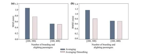
Fig.12 Comparison between methods of averaging and averaging plus smoothing: a MAE; b RMSE
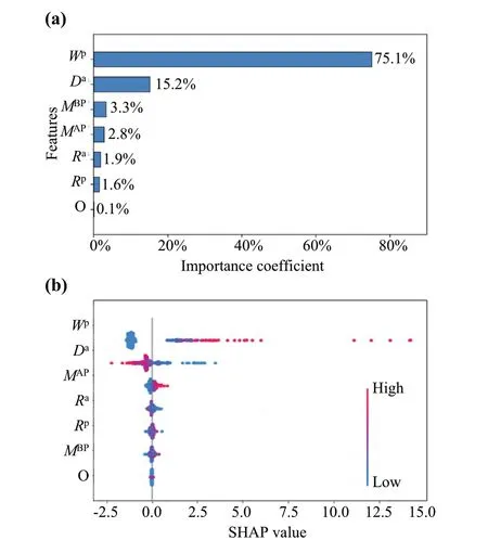
Fig.13 a The feature importance and b the SHAP value of features
Figure 13 shows the feature importance and SHAP value.From Fig.13a, we can observe that the planned dwell time and arrival delay are the most important two features, cumulatively accounting for over 90% of the output.The train overtaking relationship has the least essential impact on the output, accounting for less than 0.1% of the output.This result is probably because the research objective is a highspeed railway line.In high-speed railway lines, changing train orders were hardly taken in real-time dispatching.
Figure 13b shows the SHAP values of the model.In Fig.13, variables are ranked in descending order based on their average SHAP values in the vertical axis; the horizontal axis shows the exact SHAP value associated with each observation, i.e., negative or positive to the output; the color shows whether a variable is high (in red) or low (in blue).From Fig.13b, we can observe that: (1) theWpandDaalso exhibit the most important influences on the output; (2) theWphas positive impacts on the output, i.e., longer planned dwell time resulting in longer actual dwell time, and theDahas negative impacts on the output, i.e., long train delays resulting in shorter actual dwell time.The results are intuitive, as long planned dwell time mostly mean more passengers.In addition,supplement time in stations will be used to recover delays,leading to shorter dwell time in long-delay situations.
6 Conclusions and discussions
We propose a train dwell time prediction model for realtime train operation control in the present study.We first investigated the influence factors of train dwell time and the challenges due to the data types and data distributions.To improve the performance of the dwell time prediction model on the dataset, an averaging mechanism is proposed.The averaging mechanism in the present study is based on multiple state-of-the-art base predictors (four in our study), enabling the proposed model to address the weaknesses of different machine learning models.The performance of the proposed model is proven to be better than that of the corresponding single-base predictor on different prediction horizons regarding predictive errors and variances.In addition, we found that the existing dwell time prediction models cannot consider real-time passenger flow information.We thus used a dynamic updating/smoothing technique to improve the performance of the proposed prediction model based on a smoothing technique and real-time passenger data.The results show that dynamic updating can improve predictive accuracy in situations when passenger amounts soar or plunge.Based on the proposed tree-based predictors, a feature importance analysis shows that the planned dwell time and arrival delay are the two most important factors to dwell time.However, planned times have positive influences, whereas arrival delays have negative influences.
Train dwell time, train running time, and train headway are critical components of train operations.They are easily influenced by unexpected factors (e.g., bad weather,infrastructure failure), leading to train delays and affecting the whole train operation process.Operators usually need to calculate the minimum needed train dwell time based on given parameters (e.g., the number of station tracks,passenger flow, and technical operation times) to make the railway schedules in the timetable planning process.Predicting train dwell time provides proactive decisions for operators in the timetable planning process and under train-delay situations, but for passengers to replan their journeys.For example, traffic controllers can consider the estimated dwell time and the reordering actions for more train delay recoveries, as they can let the trains with longer estimated dwell time be overtaken by other passing trains or trains with shorter estimated dwell time.Passengers can know the expected train arrival and departure delays with the estimated train dwell time.
The future directions will be focused on the explorations of train dwell time prediction, considering more detailed factors.For example, considering the number of train doors,the lengths of the trains, and the combination of multiple factors with types of disturbances are the main directions of our interests.In addition, as the critical components of train operations, the running time model and headway model by considering the temporal and spatial differences,and the influence of disturbances is also one of our interests.Finally, one of the main disadvantages of the present study is the limited passenger data.Therefore, one of our future research directions is to investigate the performance and robustness of the dwell time prediction model over data volume.
Acknowledgements This work was supported by the National Natural Science Foundation of China (No.71871188).
Open Access This article is licensed under a Creative Commons Attribution 4.0 International License, which permits use, sharing,adaptation, distribution and reproduction in any medium or format,as long as you give appropriate credit to the original author(s) and the source, provide a link to the Creative Commons licence, and indicate if changes were made.The images or other third party material in this article are included in the article's Creative Commons licence, unless indicated otherwise in a credit line to the material.If material is not included in the article's Creative Commons licence and your intended use is not permitted by statutory regulation or exceeds the permitted use, you will need to obtain permission directly from the copyright holder.To view a copy of this licence, visit http:// creat iveco mmons.org/ licen ses/ by/4.0/.
杂志排行
Railway Engineering Science的其它文章
- A strategy for lightweight designing of a railway vehicle car body including composite material and dynamic structural optimization
- Temperature field test and prediction using a GA-BP neural network for CRTS II slab tracks
- Electromagnetic interference assessment of a train-network-pipeline coupling system based on a harmonic transmission model
- A rigid-flexible coupling finite element model of coupler for analyzing train instability behavior during collision
- Inconsistent effect of dynamic load waveform on macroand micro-scale responses of ballast bed characterized in individual cycle: a numerical study
- Influence of train speed and its mitigation measures in the shortand long-term performance of a ballastless transition zone
