Unpacking the black box of deep learning for identifying El Niño-Southern oscillation

Yu Sun,Yusupjan Habibulla,Gaoke Hu,Jun Meng,Zhenghui Lu,Maoxin Liu and Xiaosong Chen

1 School of Systems Science/Institute of Nonequilibrium Systems,Beijing Normal University,Beijing 100875,China

2 School of Physics and Technology,Xinjiang University,Wulumuqi 830017,China

3 School of Science,Beijing University of Posts and Telecommunications,Beijing 100876,China

4 National Institute of Natural Hazards,Ministry of Emergency Management of China,Beijing 100085,China

Abstract By training a convolutional neural network (CNN) model,we successfully recognize different phases of the El Niño-Southern oscillation.Our model achieves high recognition performance,with accuracy rates of 89.4% for the training dataset and 86.4% for the validation dataset.Through statistical analysis of the weight parameter distribution and activation output in the CNN,we find that most of the convolution kernels and hidden layer neurons remain inactive,while only two convolution kernels and two hidden layer neurons play active roles.By examining the weight parameters of connections between the active convolution kernels and the active hidden neurons,we can automatically differentiate various types of El Niño and La Niña,thereby identifying the specific functions of each part of the CNN.We anticipate that this progress will be helpful for future studies on both climate prediction and a deeper understanding of artificial neural networks.

Keywords: deep learning,El Niño-Southern oscillation,convolutional neural network,interpretability

1.Introduction

Deep learning [1–6] has emerged as a powerful and adaptive paradigm for handling complexity and acquiring abstract representations from data.It has led to groundbreaking advancements in various fields such as Earth system science[7–12],biology[13,14],finance[15],transportation[16,17],and more.However,the interpretability [8,18–24] of deep learning models,often referred to as ‘black boxes’ [25–27],remains a pressing concern.Deriving human-comprehensible insights from these models [28–31] is crucial for a deeper understanding and generating domain knowledge.Noteworthy interpretation skills,including layerwise relevance propagation [24,32–34],saliency maps [35–38],optimal input [39],and others,have been employed in efforts to unravel the inner mechanisms of deep learning models.However,these existing approaches predominantly focus on identifying the empirical features that contribute to the model’s output rather than delving into the causal clues within the black box itself [8,40–43].

The El Niño-Southern Oscillation (ENSO) is a wellknown interannual climate variability phenomenon [44,45].ENSO is characterized by abnormal warming or cooling in the equatorial central and eastern Pacific region,and its anomalous state has far-reaching meteorological impacts on a global scale [46–48].Numerous studies have employed a variety of deep learning architectures to analyze and forecast the evolution of ENSO [9,34,49–51].For example,Ham et al proposed a deep ensemble prediction framework for forecasting El Niño events using CNNs with improved prediction accuracy compared to traditional statistical models[9].While this study contributes to ENSO prediction accuracy,it has several potential shortcomings.The primary limitation lies in the limited interpretability of CNNs,which hinders a clear understanding of the model’s decision-making process.In addition,the reliance on data quality may also affect the confidence of the predictions.

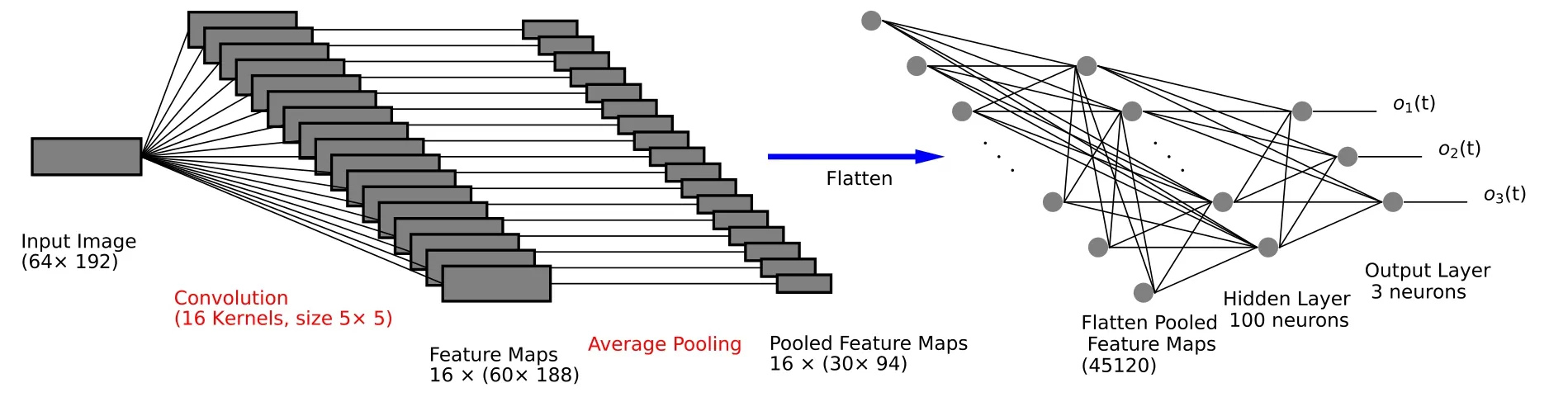
Fig.1.Architecture of the CNN model used in this study.Our CNN architecture comprises a convolutional layer with 16 convolution kernels of size 5×5.These kernels function as filters,processing the input image through element-wise multiplications and aggregating activation feature maps.Subsequently,the feature maps undergo a 2×2 average pooling layer,reducing their size by aggregating values within local neighborhoods.The pooled feature maps are then flattened and fully connected to a hidden layer consisting of 100 neurons.Finally,the neurons in the hidden layer are connected to a fully connected output layer with 3 neurons.

Deep learning models can be viewed as compositions of constituent units called neurons[1–3],with the representation encompassing both individual neuron parameter features and the collective behavior arising from their activation states.Investigating individual neurons and their activation states is of fundamental importance to achieve a comprehensive understanding of the representation.Moreover,the complexity of deep learning models is intrinsically linked to the complexity of the learning tasks they tackle,as exemplified by DeepMind’s research [52].When a deep learning model exhibits perfect performance in solving a specific task,it implies that the model’s representation encodes the task’s intrinsic features [53].Therefore,with improved measurability and transparency offered by deep learning models,the complexity inherent in these systems should not serve as an excuse to avoid studying them.Instead,it should serve as motivation to investigate further.

Based on this perspective,a methodology is proposed to analyze the inner representation of deep learning models.We use it to elucidate the inner workings of a convolutional neural network(CNN)model designed to classify ENSO.Our deep learning task focuses on classifying different phases of ENSO based on near-surface air temperature.The welltrained model demonstrates precise identification of distinct ENSO phases.Analysis of the internal model representation reveals a condensed and simplified parameter structure,improving our understanding of each component’s taskspecific function.Remarkably,this parameter structure enables clear differentiation between eastern Pacific (EP)and central Pacific(CP)El Niño patterns,as well as weak and extreme La Niña patterns,shedding light on the crucial features of this natural phenomenon.

This study serves as a rudimentary model for delving into the black boxes of complex systems,providing preliminary insights and inspiration for harnessing the power of deep learning to comprehend phenomena within complex systems.Moreover,we firmly believe that the fundamental perspective and methodology employed in this study possess the potential to be extended to more intricate models,owing to the inherent nature of complexity that is shared among diverse systems.

2.Data and methods

2.1.Data

The aim of our learning task is to identify different phases of the ENSO based on the images of near-surface air temperature.ENSO is a basin-scale phenomenon that involves coupled atmosphere-ocean processes.It consists of three phases:El Niño,La Niña,and the normal phase.El Niño and La Niña refer to irregular warming and cooling of the equatorial central and eastern Pacific region.To define the phases,we conventionally employ the Oceanic Niño Index (ONI,https://origin.cpc.ncep.noaa.gov/products/analysis_monitoring/ensostuff/ONI_v5.php,accessed on 31 May 2019)[54],which is a three-month running mean of sea surface temperature anomaly(SSTA)in the Niño3.4 region (5°N–5°S,170°W–120°W).According to NOAA’s definition,for a full-fledged El Niño or La Niña event,the ONI must exceed+0.5°C or–0.5°C for at least five consecutive months.

We utilize near-surface(2 m)air temperature data as input and assign the corresponding ENSO phase as the label.The daily near-surface(2 m) air temperature data is obtained from the National Centers for Environmental Prediction-National Center for Atmospheric Research (NCEP-NCAR) Reanalysis[55] (https://psl.noaa.gov/data/gridded/data.ncep.reanalysis.html,accessed on 31 May 2019),presented as grids with a latitude-longitude interval of 1.9° × 1.875°.Our region of interest spans from 60°S to 60°N,consisting of a total of N=64 × 192 grids.We label the ENSO phases using a threedimensional vector c(t),which is equal to(1,0,0)for El Niño,(0,1,0) for La Niña,and (0,0,1) for the normal phase.

For the purposes of training and validation,we split the dataset into two parts.The training dataset covers 1 January 1950 to 31 December 1999,and consists of a total of 18,262 d.The validation dataset spans 1 January 2000 to 31 December 2018,and consists of a total of 6,490 d.To filter out the fluctuations of short time scales in the data,we applied a 30 d sliding average with a sliding step of 1 d.To validate the robustness of our analysis,the daily data without the sliding average is applied for training as a comparison in appendix B.

We denote the surface temperature of grid i at time t as Si(t) with the average

where t0is 1 January 1950,t1is 31 December 1999,and T represents the total number of days in this period.The temperature fluctuation of grid i at time t is given by

The root mean square deviation for grid i is calculated as

Considering the significant differences in temperature fluctuations across different regions,we standardize the data for each grid i using

The input to the neural network is represented as

2.2.Convolutional neural network

In this study,we employ CNN,a classical and wellestablished deep learning architecture,to address the task of ENSO phases recognition within the deep learning paradigm,as shown in figure 1.Our specific CNN architecture consists of a convolutional layer comprising 16 convolution kernels,each with a size of 5×5.These kernels act as filters,transforming the input image by performing element-wise multiplications and subsequently aggregating the resulting activation feature maps.These feature maps then undergo a 2×2 average pooling layer,reducing the size of the feature maps through coarse-graining values within 2×2 local neighborhoods.The pooled feature maps are then connected to a fully-connected hidden layer comprising 100 neurons.Finally,the neurons within the hidden layer are connected to a fully-connected output layer,housing only 3 output neurons.This output layer facilitates the decision-making process,providing the output vector o(t)=(o1(t),o2(t),o3(t)),where o1(t),o2(t),and o3(t) represent the predicted intensities for El Niño,La Niña,and normal phases,respectively.

The neuron parameters are randomly initialized before the training process,and the meaningful representation develops through the training process.Following the convention in deep learning classification tasks,cross-entropy loss function is utilized to quantify the discrepancy between the softmax normalized outputs and the labels.The training objective is to minimize the overall discrepancy by adjusting the neuron parameters.To mitigate overfitting,we incorporate L2parameter regularization [3] by adding a penalty term to the loss function.If a significant discrepancy in accuracy arises between the training and validation datasets,training with increased L2regularization strength is necessary to ensure satisfactory performance on the validation data.

2.3.Unpacking the black box

Unpacking the black box involves examining neuron parameters and activation states.The importance of neuron parameters is assessed based on their significance.Understanding the spatial distribution of parameters and sorting them accordingly provides valuable insights,highlighting the key components that drive the inner workings of the black box.Additionally,a deep understanding of the collective behavior of activation states is also essential for comprehending the black box.

3.Results

3.1.Identification of ENSO phases

Impressive accuracy results have been achieved for both the training and validation datasets through sufficient training.The accuracy stands at 89.4% for the training datasets and reaches 86.4%for the validation datasets.From the validation datasets,we obtain the prediction o(t)=(o1(t),o2(t),o3(t)),which refers to the El Niño,the La Niña,and normal phases,respectively.The ENSO phases are identified by the largest output.In addition,we try to quantify the significance of the identified ENSO phase.The significance is related to the standard deviation

which is depicted in figure 2(a).For some states with significance R(t)＜10 and persistence in an ENSO phase for less than 2 months,their phase is defined as that of the previous states.

From figure 2(a),we can see that all El Niño events since 2000 have been correctly identified.The very strong El Niño event from 2015 to 2016 has been classified with a very large R(t).The strong La Niña events at 1999–2000,2007–2008,and 2010–2011 have been identified with large R(t).Two misjudgments appear for the two weakest events at 2005–2006 and 2016–2017,which are indicated by small R(t) as well.

3.2.Unpacking the neural network

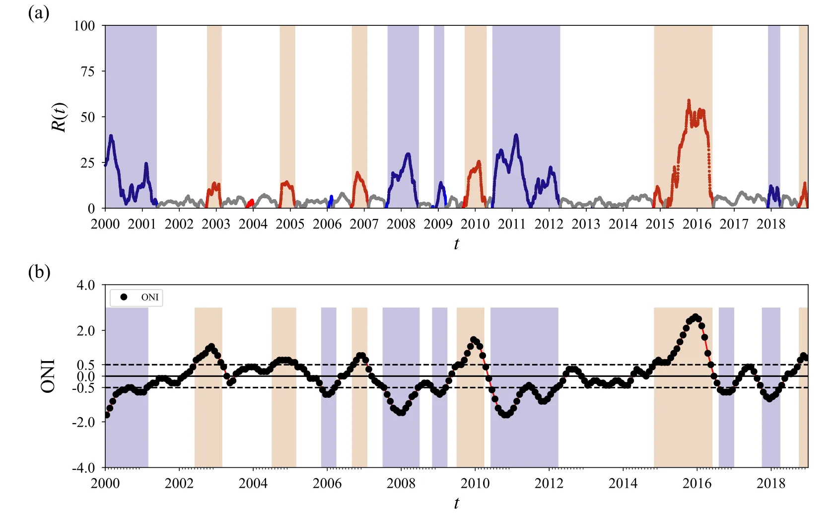
Fig.2.(a) Identification of ENSO phases and their significance for the validation dataset (2000–2018) with the El Niño,La Niña,and normal phases represented by the red,blue,and white backgrounds respectively.(b) The Oceanic Niño index (ONI) from 2000 to 2018,where the El Niño,La Niña,and normal phases are displayed with red,blue,and white backgrounds,respectively.

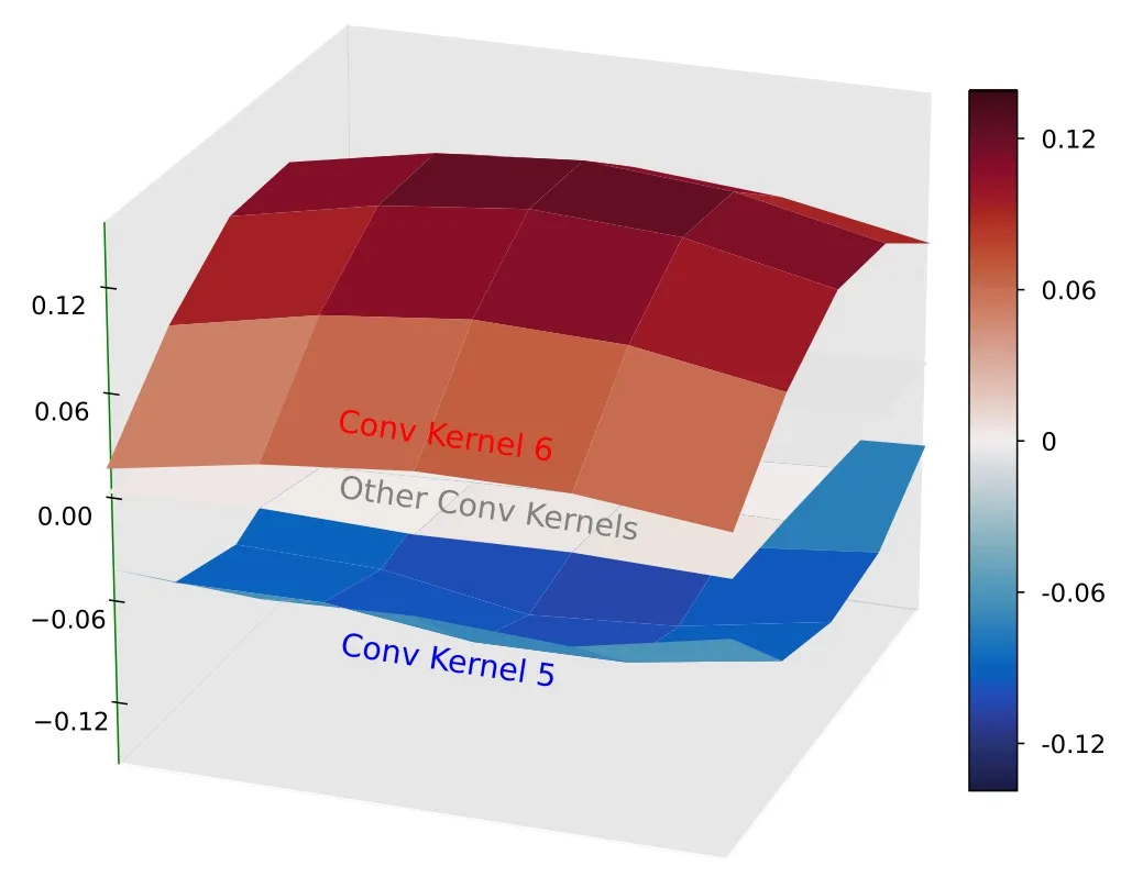
Fig.3.Visualization of the convolution kernels with their values shown as 5×5 nodes on the surface.Among the 16 convolution kernels,only kernel 5(blue surface)and kernel 6(red surface)have nonzero values.

3.2.1.Unpacking the convolutional layer.Our investigation initiates with a comprehensive examination of the convolutional layer within our CNN architecture,which consists of an ensemble of 16 convolution kernels.Notably,these kernels exhibit a remarkable degree of sparsity,with only kernels 5 and 6 emerging as the exclusive kernels manifesting notable values,as shown in figure 3.Kernel 6 presents a smooth,concave-up pattern characterized by positive values,while kernel 5 displays a smooth,convex-down pattern characterized by negative values.By comparing the output feature maps produced by each kernel with the input image,we can discern the distinct functions that these kernels serve,as demonstrated in appendix A.Kernel 6 effectively captures positive features,representing the magnitude of positive temperatures in its feature map.Conversely,kernel 5 adeptly captures negative features,representing the magnitude of negative temperatures in its feature map.The remaining convolution kernels yield null outputs,indicating that their outputs do not contribute to the final prediction.

3.2.2.Unpacking the hidden layer.In the hidden layer consisting of 100 fully-connected neurons,it is vital to identify key neurons.By prioritizing high averages and significant variations in activation output,we observe sparse activation in this layer as well.Based on this analysis,we have identified two crucial active neurons:hidden neurons 50 and 100.Each active neuron demonstrates two distinct parameter patterns,corresponding to the connection parameters linked to feature maps derived from convolution kernels 5 and 6,respectively.

The patterns observed in neuron 100 effectively capture the unique characteristics of El Niño,specifically the anomalous warming in the eastern and central equatorial Pacific.This neuron displays a selective response to positive signals,particularly in the central and eastern Pacific regions,when analyzing the positive features extracted by kernel 6(figure 4(a)).Conversely,when these regions exhibit concentrated negative features extracted by kernel 5,neuron 100 exhibits a low activation output,as shown in figure 4(b).

It is very interesting to note that these patterns inherently capture the distinct spatial patterns between the EP and the CP El Niño flavors.The EP and CP flavors are of significant importance in comprehending the El Niño phenomenon as they represent distinct anomalous temperature patterns accompanied by notable variations in regional climatic impacts [56].As shown in figure 4(a),the connection parameters associated with the feature map derived from kernel 6 exhibit an EP flavor,aligning with the maximum warming observed in the eastern Pacific near the coast of South America (see the EP El Niño pattern shown in figure 2(a) of [56]).As depicted in figure 4(b),the connection parameters linked to the feature map derived from kernel 5 exhibit a distinct CP flavor.The CP flavor corresponds to the anomalous center observed in the central equatorial Pacific and is notable for its characteristic horseshoe pattern (see the CP El Niño pattern shown in figure 5(b) of [56]).

Fig.4.(a)–(b) Visualization of nontrivial parameters for hidden neuron 100.The connection parameters associated with feature maps derived from convolution kernels 6 and 5 are visualized in (a) and (b),respectively.

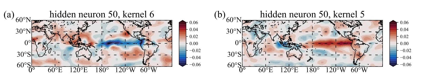
Fig.5.(a)–(b) Visualization of nontrivial parameters for hidden neuron 50.The connection parameters associated with feature maps derived from convolution kernels 6 and 5 are visualized in (a) and (b),respectively.

On the other hand,the observed patterns in neuron 50 reflect the distinctive characteristics of La Niña,specifically the anomalous cooling observed in the eastern and central equatorial Pacific.This neuron demonstrates a selective response to negative signals,particularly in the central and eastern Pacific regions,when analyzing the negative features extracted by kernel 5,as shown in figure 5(b).Conversely,when these regions exhibit concentrated positive features extracted by kernel 6,neuron 50 exhibits a low activation,as shown in figure 5(a).The connection parameters associated with Neuron 50 also display two distinctive patterns.Notably,it reveals a clear distinction between different types of La Niña patterns.Despite the lack of distinctiveness in the CP and EP types of La Niña[57],there are significant differences in spatial distribution between weak and extreme La Niña[58].Figure 5(a) shows that the connection parameters associated with the feature map derived from kernel 6 correspond to the weak La Niña pattern,while the feature map derived from kernel 5 corresponds to the extreme La Niña pattern(refer to figures 1(a)–(b)of[58]for the weak and extreme La Niña patterns).

3.2.3.Unpacking the output layer.The output layer comprises 3 output neurons,each playing an important role in predicting El Niño,La Niña,and the normal phases,respectively.Therefore,we directly refer to the three neurons as the El Niño neuron (output neuron 1),the La Niña neuron(output neuron 2),and the normal neuron (neuron 3),respectively.The contribution of hidden neurons to each output neuron is reflected in the parameters,as shown in figure 6.Sparsity is observed,with only active hidden neurons (hidden neurons 50 and 100) significantly contributing to the output neurons,consistent with the discussion in section 3.2.2.The distinct roles of these active hidden neurons can be identified based on their contributions.Hidden neuron 100 promotes El Niño prediction while inhibiting La Niña prediction,while hidden neuron 50 exhibits the opposite effect.

4.Conclusions

In this work,we employ near-surface (2 m) air temperature data from NCEP/NCAR reanalysis data to train a CNN in recognizing various phases of ENSO.Our model exhibits high recognition accuracy,with the training dataset and validation dataset achieving accuracy rates of 89.4% and 86.4%,respectively.To further understand the underlying principles behind the good performance of our neural network model,we examine the parameter distribution and activation output in the neural network.It turns out that only two sets of convolution kernels (the No.5 and the No.6) are actively contributing to the results,while others are of zero value.Thus,we can only use one of these two sets of convolution kernels (the No.5 and the No.6) to extract positivetemperature or negative-temperature features from the original input of the global temperature field,respectively.Similarly,among the total of 100 hidden layer neurons,only two neurons (the 50th and the 100th) are playing a dominant role in the model.The 100th neuron responds to El Niño features,and the 50th neuron responds to La Niña features.By analyzing the connection weight parameters between the two active convolution kernels(the No.5 and the No.6)and the two dominant hidden layer neurons (the 50th and the 100th),we found that each weight parameter represents the characteristics of a certain type of El Niño or La Niña.Therefore,we can distinguish different types of El Niño and La Niña in sufficiently clear geographical regions.For example,the four types of climate phenomena (the eastern type El Niño,the central type El Niño,the weak La Niña,and the extreme La Niña) are readily recognized according to the four connection weight parameter patterns between the two active convolution kernels and the two dominant hidden layer neurons(No.6 and the 100th,No.5 and the 100th,No.6 and the 50th,and No.5 and the 50th).This work shows that our model successfully learns and differentiates specific features of climate phenomena.We expect this progress is helpful for both future predictions of climate change and a deep understanding of the general underlying mechanism of artificial neural networks.

Acknowledgments

This work is supported by the National Natural Science Foundation of China (Grant No.12135003).We also acknowledge Jingfang Fan,Yongwen Zhang,Naiming Yuan,and Jiaqi Dong for discussions.

Appendix A.Demonstration of the effects of convolution kernels

As shown in figures A1–A5,convolution kernel 6 captures positive features,representing the magnitude of positive temperatures in its feature map.Convolution kernel 5 captures negative features,representing the magnitude of negative temperatures in its feature map.The remaining convolution kernels produce null outputs,signifying that their outputs do not contribute to the final prediction.These effects hold true for any selected dates as well.

Figure A2.Illustration of convolution kernels with the input image sampled from 1 November 2009,during the CP El Niño period.

Figure A3.Illustration of convolution kernels with the input image sampled from 1 February 2018,during the weak La Niña period.

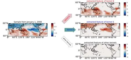
Figure A4. Illustration of convolution kernels with the input image sampled from 1 January 2008,during the extreme La Niña period.

Figure A5. Illustration of convolution kernels with the input image sampled from 1 March 2007,during the normal period.

Appendix B.Reproducibility and the robustness of results

To demonstrate the robustness and reproducibility of our study,we conduct two groups of independent parallel trainings.We use daily data from the same dataset without the sliding average to validate the analysis’s robustness.In figures B1–B3,we compare the monthly predictions between the original training and the two parallel trainings.In figures B4–B6,we compare the outputs of active hidden neurons between the original training and the two parallel trainings.Similarly,in figures B7–B9,we compare the outputs between the original training and the two parallel trainings.The parameters for the two parallel trainings are shown in figures B10–B12 and figures B13–B15,respectively.During the parallel trainings,we observed that training with daily data resulted in the emergence of an additional active neuron in the hidden layer.By examining the output of this neuron,we discovered that it exhibited relatively low variability and followed an annual cycle,as shown in figures B5(c) and B6(c).This may be caused by the stronger fluctuations and volatility inherent in the daily data.

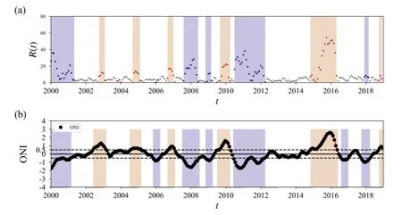
Figure B1. The monthly predictions for the validation dataset (2000–2018).

Figure B2. The monthly predictions for the validation dataset (2000–2018) in parallel training 1.

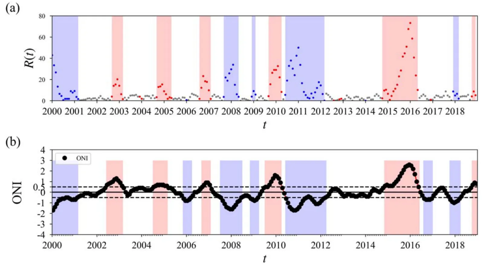
Figure B3.The monthly predictions for the validation dataset (2000–2018) in parallel training 2.

Figure B4.The nontrivial outputs of hidden layer for the validation dataset (2000–2018).

Figure B5.The nontrivial outputs of hidden layer for the validation dataset (2000–2018) in parallel training 1.

Figure B6. The monthly predictions for the validation dataset (2000–2018) in parallel training 2.

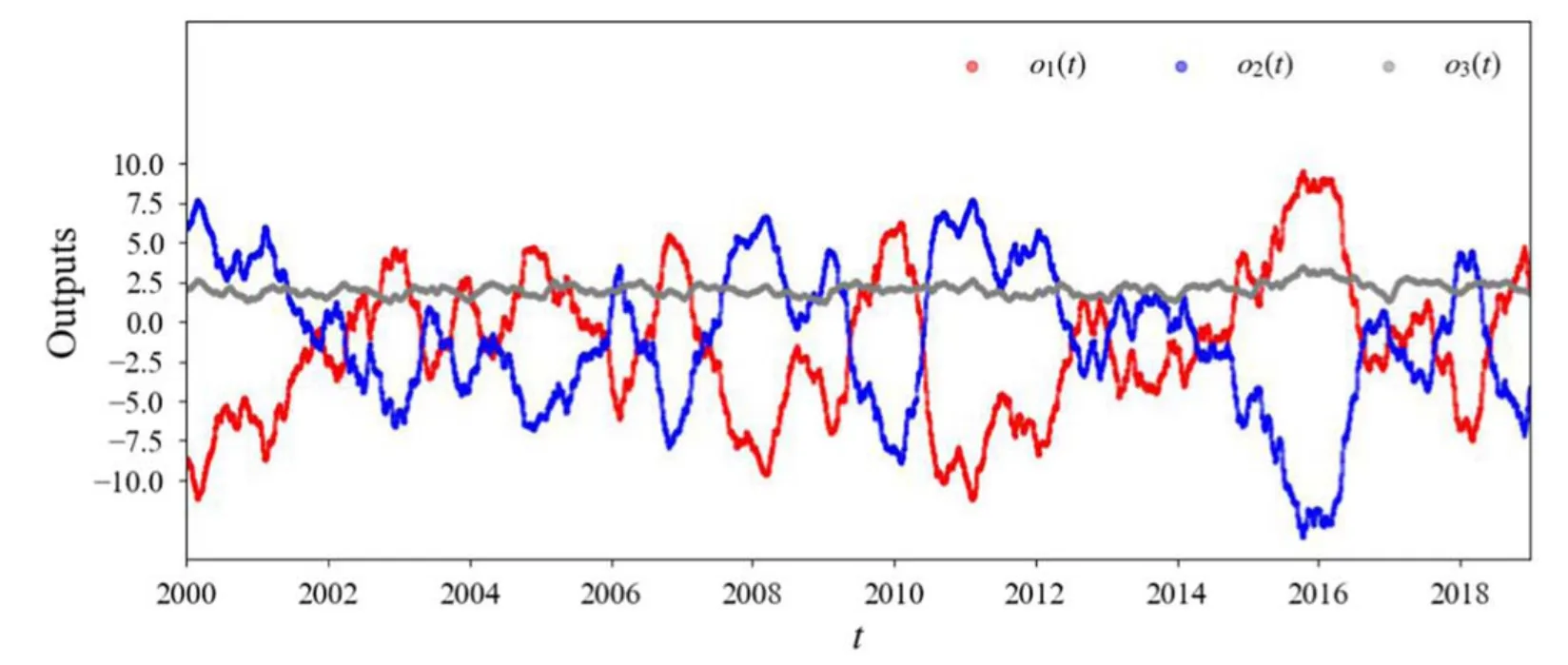
Figure B7.The outputs of output layer for the validation dataset (2000–2018).

Figure B8. The outputs of output layer for the validation dataset (2000–2018) in parallel training 1.

Figure B9.The outputs of output layer for the validation dataset (2000–2018) in parallel training 2.

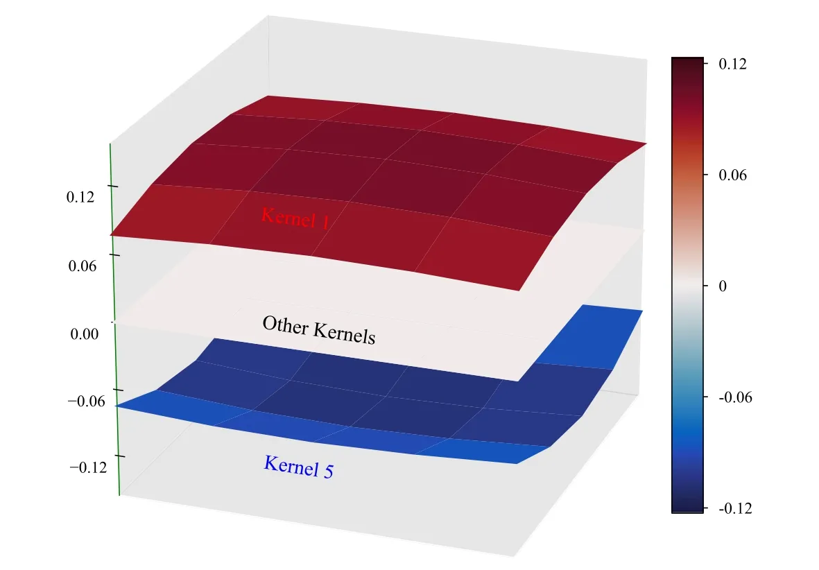
Figure B10.Visualization of the convolution kernels in parallel training 1 with their values shown as 5×5 nodes on the surface.

Figure B12.Visualization of the parameters for output neurons in parallel training 1.

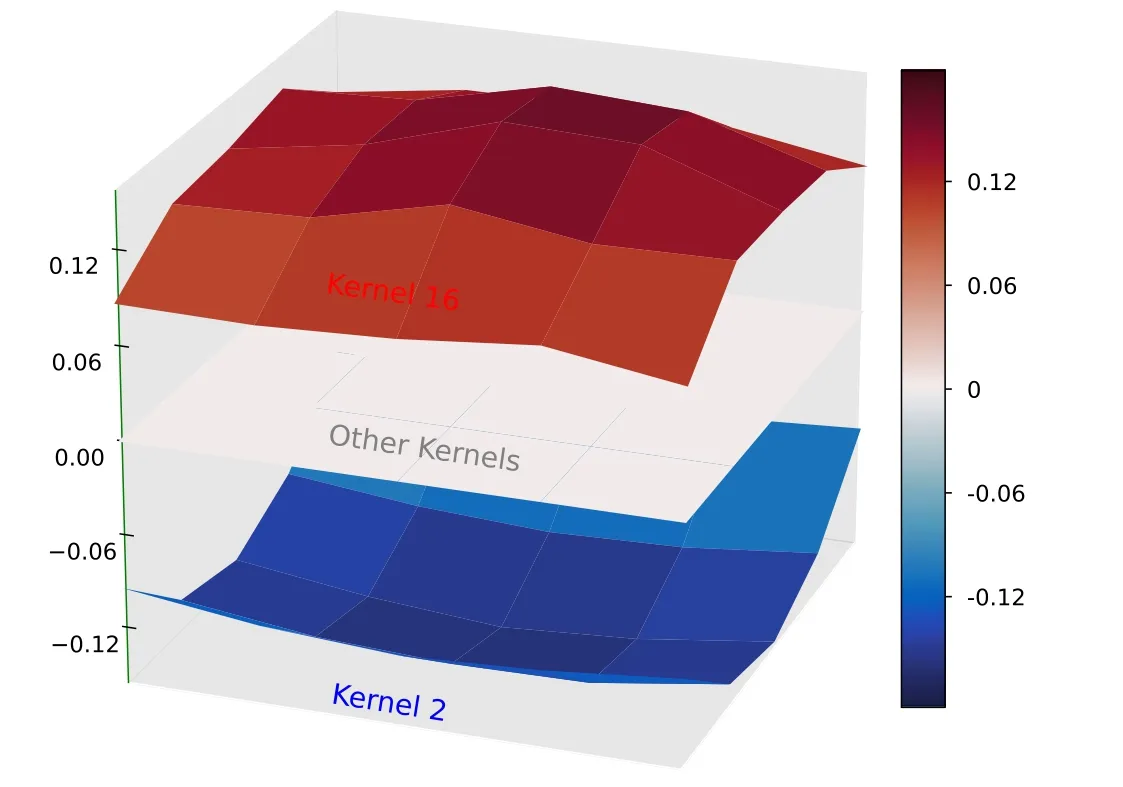
Figure B13.Visualization of the convolution kernels in parallel training 2 with their values shown as 5×5 nodes on the surface.

Figure B14.Visualization of nontrivial parameters in the hidden layer of parallel training 2.

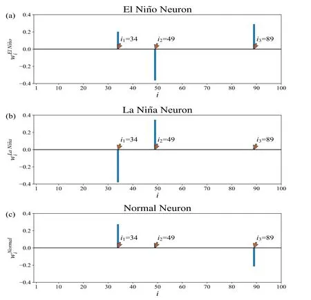
Figure B15.Visualization of the parameters for output neurons in parallel training 2.

Appendix C.Details about the CNN

C.1.Neurons and convolution kernels

A neuron extracts the feature from its input.We have depicted the workflow of a neuron in figure C1.The ReLU function which is used as the activation function in a neuron is shown in figure C2.Convolution kernels act as filters,transforming the input image by performing element-wise multiplications and subsequently aggregating the resulting activation feature maps.We present the schematic diagram of convolution kernels in figure C3,illustrating two kernels of size 3×3 as an example.

C.2.Loss function and L2parameter regularization

In the training process,the cross-entropy function is used to measure the loss at time t

Here,c(t) denotes the label,and p(t) denotes the softmax normalized output with

The training is essentially a fitting process which minimizes the total loss by tuning neural network parameters.To suppress overfitting during the training process,L2parameter regularization is used.This method updates the loss function to be minimized from loss(t) to

is referred to as the L2parameter for neuron m,and α is the factor used to control the strength of L2parameter regularization during the training process.

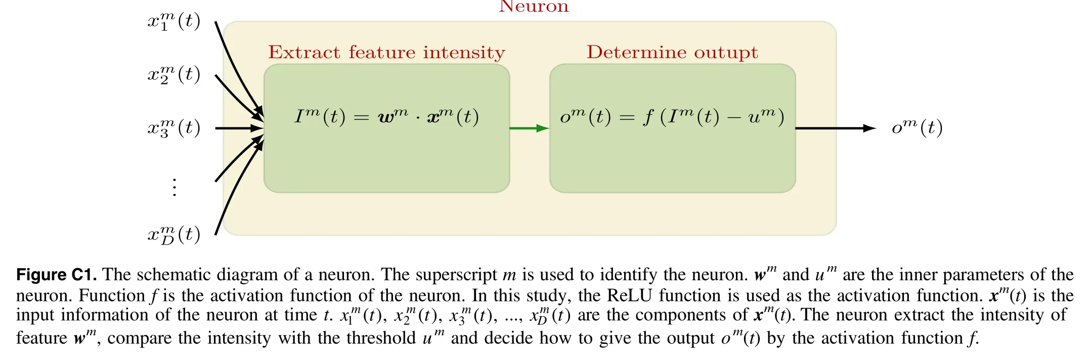
Figure C2. The ReLU function. ReLU(x )=max(x,0).

Figure C3.The schematic diagram of convolution kernels.This is an example for two convolution kernels of size 3×3.These convolution kernels act as filters,transforming the input image by performing element-wise multiplications and subsequently aggregating the resulting activation feature maps.