LitePIG: a lite parameter inference system for the gravitational wave in the millihertz band

Renjie Wang and Bin Hu,∗

1 Institute for Frontier in Astronomy and Astrophysics,Beijing Normal University,Beijing,102206,China

2 Department of Astronomy,Beijing Normal University,Beijing,100875,China

Abstract

We present a Python based parameter inference system for the gravitational wave (GW)measured in the millihertz band.This system includes the following features:the GW waveform originated from the massive black hole binaries (MBHB),the stationary instrumental Gaussian noise,the higher-order harmonic modes,the full response function from the time delay interferometry and the Gaussian likelihood function with the dynamic nested parameter sampler.In particular,we highlight the role of higher-order modes.By including these modes,the luminosity distance estimation precision can be improved roughly by a factor of 50,compared with the case with only the leading order (ℓ=2,|m|=2) mode.This is due to the response functions of different harmonic modes on the inclination angle are different.Hence,it can help to break the distance-inclination degeneracy.Furthermore,we show the robustness of testing general relativity (GR) by using higher-order harmonics.Our results show that the GW from MBHB can simultaneously constrain four of the higher harmonic amplitudes (deviation from GR) with 95% confidence level ofc21=,c32=-,c33= and c44=,respectively.

Keywords: gravitational wave astronomy,data analysis,parameter estimation

1.Introduction

Gravitational waves(GWs)from compact binary coalescence(CBC) events open a new observational window to explore the nature of the Universe.The LIGO[1]-Virgo[2]-KAGRA[3] (LVK) scientific collaboration has detected 90 GWs from CBCs up to the end of the third observing run(O3)[4].These CBC events can be used to study the properties of stellarmass black holes and neutron stars.The future space-borne gravitational wave observatory,such as the Laser Interferometer Space Antenna (LISA) [5],Taiji [6] and TianQin[7] will be able to measure the GW events in the millihertz band,which contains many sources including massive black hole binaries(MBHB)[8],extreme mass-ratio inspiral[9]and white dwarf binaries [10],etc.MBHBs are one of the main scientific goals of the space-borne gravitational wave observatory because of their high detection significance.Hence,these objects are suitable for precise astrophysics and cosmology studies [11-14].

In general,GW signals are the superposition of multiple harmonic modes [15].The dominant harmonic is the (ℓ,|m|)=(2,2) harmonics.Compared with the (2,2) mode,the higher-order harmonics are much weaker.Two important intrinsic parameters affecting the amplitude of each higherorder mode are mass ratio and total mass [16].The spin parameter entering at higher post-Newtonian order has a significant impact on the waveform [17].The higher-order harmonics can bring in new dependencies on the mass ratio,component spins,and inclination angle into the waveform[18-20].The importance of including these higher-order harmonics in the waveform is that one can break the degeneracy between the luminosity distance and inclination angle[21,22].Recent observations of GW190412 [23] and GW190814 [24],which were generated from CBCs with significantly asymmetric component masses,confirm the presence of higher-order harmonics emission at a high confidence level.The network with two 3G ground-based detectors is promising to detect higher-order harmonics [18].Furthermore,including higher-order harmonics can increase the signal-to-noise ratio for Intermediate mass ratio inspiral(IMRI) binaries and improve the measurement of IMRI source properties[25].For an equal-mass neutron star merger system at a distance similar to GW170817,the inclusion of higher-order modes leads to improvements in the distance and inclination and allows for percent-level measurements of the Hubble parameter [26].Further,the higher-order harmonics can be used to test general relativity (GR) [27,28].

In our work,we present a Python based parameter inference system for the GW measured in the millihertz band.In particular,we highlight the importance of including the higher-order harmonics in the parameter estimation.In section 2,taking LISA as an example,we demonstrate the methodology of GW signal generation,the time delay interferometry (TDI)response and the low-frequency approximation,which is currently adopted.In section 3,we describe the parameter likelihood construction as well as the sampling method.In section 4,we show the luminosity distance parameter estimation from MBHB as an example.Furthermore,we show the capability of testing GR with higher-order harmonics.We draw the conclusion at the end.

2.LISA response and waveform generation

In this section,we will take LISA as an example to illustrate our methodology of GW waveform generation.

2.1.The GW signal

The GW waveform in the transverse-traceless gauge is described by the two polarizations h+,h×.Furthermore,h+,h×can be decomposed into the spherical harmonic modes,hℓm,by using the spin-weighted spherical harmonics as functions of the inclination angle ι and coalescence phase φc.The waveform can be expressed as

The spin-weighted spherical harmonics for the modes−2Yℓm(ι,φc) can be found in appendix A of [16].The dominant harmonic is h22,all the others are called higher-order modes.Furthermore,one can translate the mode decomposition equation (1) into the Fourier domain

For non-precessing binary system,an exact symmetry relation between modes allows us to write

Therefore,we can further write

with

In the Fourier domain,we often use the one side frequency spectrum,namely either keep the positive or the negative parts depending on the sign of m [16,29,30].This approximation is valid in particular where the stationary phase approximation can be used.Hence,we assume

and neglect modes hℓ0.With this approximation we can obtain explicit expressions for positive frequency modes

The GW waveform can be expressed as a superposition of individual harmonics.Figure 1 shows the dependence of the modes on inclination.For the (2,2) mode,the plus polarization peaks at face-on configuration,while(2,1),(3,3)and(4,4)modes vanish at face-on.The amplitude of(3,2)modes can reach a maximum at both face-on and edge-on.Similarly,the amplitude of the cross polarization dependence on the inclination angle is different for each mode.Because of these differences,the inclination measurement can be improved when higher-order modes are measured [16].Therefore,the well-known degeneracy between distance and inclination angle can be broken.

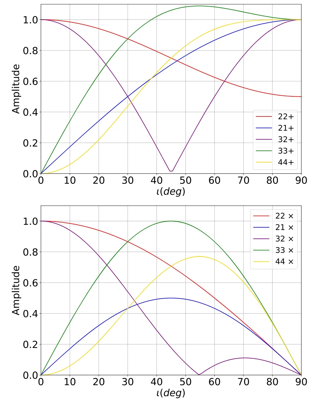
Figure 1.The amplitude of each harmonic as a function of the inclination ι.The red,blue,purple,green and gold lines denote the amplitude of some harmonics including the dominant modes ℓ=|m|=2 and a set of higher-order harmonics,(ℓ,|m|)=(2,1),(3,3),(3,2),(4,4).The first row is the result of the plus polarization while the second row is for the cross polarization.

2.2.Time delay interferometry (TDI): full response

For ground-based laser interferometers,such as LIGO [1],one can keep the same arm length up to the picometer level.Hence,the laser frequency noise can be cancelled very precisely.However,the spaceborne GW observatory will have much longer arm lengths.Compared to the ground-based interferometers,the GW space mission will be impossible to maintain equal arm lengths between spacecraft pairs.Because of the dynamics of mission orbit,the laser frequency noise cannot be cancelled to the level of measuring GW signal.For a GW space mission,the variation of the absolute arm has a typical value of 1%.To exactly cancel the laser frequency noise,the TDI technique is proposed[31].TDI had been well studied for the first-generation [32,33] and the second-generation [34].

The TDI technique is used to construct a new set of observables from delayed combinations of ysrto cancel the laser frequency noise.We assume the LISA arm lengths are all constant and equal to L.The TDI operation can construct data set with an effectively equal arm length.The laser frequency stability in the TDI data will qualify the requirement of the GW measurement.A constant 1% distance error can be resolved by the TDI technique.Hence,we can approximately assume an equal arm length.This is the standard first order approximation adopted by the community.Using the notation ysr,nL=ysr(t −nL),the first-generation TDI observable X is given by [29,34]

The other two observables Y and Z are obtained by cyclic permutation.The first-generation TDI observables (X,Y,Z)are correlated in their noise properties.They can be transformed into uncorrelated observables (A,E,T).Thus,the second-generation TDI observables A,E and T are expressed as

These channels are independent and uncorrelated.

The source frame waveforms can be represented as a combination of harmonics with the amplitude A(f)and phase Ψ(f)

Currently,there are five harmonics included in the IMRPhenomXHM template [35],namely (ℓ,|m|)=(2,2),(2,1),(3,3),(3,2),(4,4).A complex transfer function T(f,tℓm(f)) is used to transform the source-frame waveform into the TDI observables[29,30].This function is determined by the extrinsic parameters(ι,λ,β,ψ,φ0,t0).Because of the evolution of the LISA constellation,the transfer function is temporal-and frequency-dependent.The time-frequency dependence for each harmonic,tℓm(f) is defined by the stationary phase approximation (SPA)

The signal of each harmonic and for each TDI channel is given by

Figure 2 shows the characteristic strain for each harmonic modein the frequency domain.The(2,2)modeis the most dominant one and is followed by (3,3) and (2,1),sequentially.These curves are the theoretical template,the observation response function has not yet been added.

Figure 2.Characteristic strain of each harmonic mode.This displays the amplitude of each mode using the IMRPhenomXHM waveform template.Note that the plot displays the theoretical signal without convolving the response function.The black dotted line is the LISA sensitivity curve from [36].

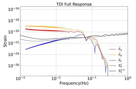
Figure 3.The characteristic strain in the three TDI channels.The red,orange and blue curves represent the characteristic strain of the signals defined by equation(24):=f ()∣.The black solid and dotted curves show the characteristic strain with the reduced noise PSDf () from equation (25).

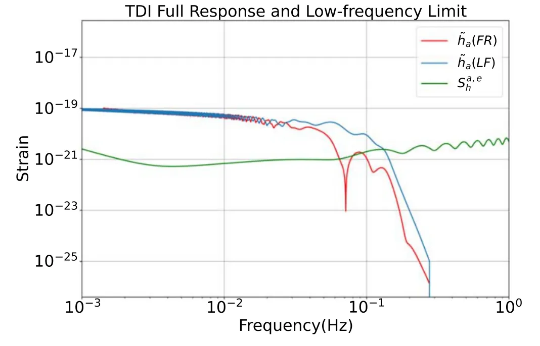
Figure 4.The characteristic strain for the A channels.The red curve represents the characteristic strain of the full response signals defined by equation (24) :=∣∣.The blue curve shows the characteristic strain using the low-frequency limit,defined by equation (27).The green solid curves show the characteristic strain with the reduced noise PSDf () from equation (25).

To compensate for the fast oscillatory in the high frequency range and avoid the numerical instability,we can rescale the TDI observables by prefactors which are common to both signal and noise [29].Thus,the TDI channels in the frequency domain can be written as

Factoring out the same sine square function from the noise power spectral density (PSD)

the reduced PSD reads

where Spmis the test-mass noise PSD and Sopis the optical noise PSD.The corresponding values for LISA can be found in [37].It is also useful to introduce the following notations

Thus,we can define a noise PSD associated with the TDI observables (24) as

Moreover,the characteristic noise strain can be defined to be

In figure 3,the solid curves show the characteristic strain(24)and the reduced noise PSD (25) for three TDI channels.One can see that the A channel is similar to the E channel,while the T channel is noise dominated.

2.3.The low-frequency limit

Though we can apply the full response to perform parameter estimation,it will be useful to consider some limits to simplify calculations.Here,we use the low-frequency approximation to the LISA response.When f ≪fL=1/L=0.12 Hz[29],the T-channel can be neglected.And in this low-frequency approximation,the response for the other two TDI observables in equation (24) are given by

which is similar to the ground-based detectors.The functionsare

For ψL=0,one has

where the LISA-frame sky position angle λL,βLand the polarization angle ψLare given by

with α=2π(t −tref)/1yr.trefis a reference time for the initial position and we assume tref=0.

The LISA response is both time-and frequency-dependent.In the low-frequency limit,because of the motion of the LISA constellation,the time dependency enters both into the Doppler phase term and into the time-dependent LISA-frame angles(λL,βL,ΨL)[29].Here,we consider the MBHB signals are short,eg.less than a few days.The orientation and position of the LISA constellation in the orbit are barely changed during the GW detection period.In the work,we consider the low-frequency limit and neglect the LISA motion,effectively freezing the LISA constellation in the orbit.We treat the LISA-frame angles (λL,βL,ΨL) as constants and neglect both the time and frequency dependency in the response.In this case,the response is similar to two LIGO-type detectors.The transfer function is just a constant factor.This approximation can be useful to analytically understand the degeneracies that occur when using the more complicated full response.For the short-duration MBHB merger events,it is a reasonable approximation.

The derivation of the above equation can be found in the literature [29].To validate the low-frequency approximation,we compare the full response TDI observables with the one using low-frequency approximation.In figure 4,the red curve shows the full response for the TDI channel ha,defined by equation (24),which is the same as the red solid curve in figure 3.The blue curve shows the TDI channel hausing the low-frequency approximation.We only show the haTDI channel because the hechannel is similar and the T channel can be neglected at low frequencies.In the low-frequency band,f<10−2Hz,the difference between the TDI using the low-frequency approximation and the full-response results is tiny.However,when f>10−2Hz,the difference becomes larger,especially at about 0.1 Hz where the difference arises.In this paper,we perform our analysis in the frequency range between 10−3Hz and 10−2Hz,in which the low-frequency approximation is completely valid.

3.Bayesian methods for massive black hole binary

In this section,we will first introduce the likelihood construction,and then the dynamic nested sampling methods.Bayesian methods are used to estimate the parameters of GW events.In general,the GW data d(t) is a superposition of noise n(t) and a possible signal h(t)

In our analysis,we will consider the low-frequency limit and simulate the rescaled signals according to equation (24).

Besides the waveform in each TDI channel,we also need the noise in each channel.We use the tdi package3 https://lisa-ldc.lal.in2p3.frfrom the LISA Data Challenges Working Group software collection to generate the PSD in each channel,.According to the definition of equation(25),we can obtain the reduced noise PSD,.The noise is generated by the public pycbc code[38].For simplicity,one can assume that the noise in the time domain is Gaussian and stationary.Under this assumption,the noise in the frequency domain is Gaussian with zero mean and is characterised by the noise PSD,Therefore,we can generate the data set by summing the signal and noise in each TDI channel.

Using the Bayesian methods,the posterior distribution can be determined as

where Λ is the model of the GW signal and Θ are the parameters of this model.p(Θ|λ) represents the prior probability and the likelihood p(d|Θ,Λ)is the probability of the observed data d(t)given the waveform model Λ and a set of parameters Θ.In the low-frequency limit,the likelihood is given by

where the inner product is really the sum of the inner products over all the TDI channels rescaled by equation (24)

Sha,e(f) is noise PSD given by equation (25).The optimal signal-to-noise ratio (SNR) is given by

In this work,we use the reduced TDI templates equation(24)and the analytic function Sihgiven by equation(25).The noise PSD for TDI observables haand heare identical.

Higher-order modes can be used to break the degeneracy between the distance and inclination of the binary coalescence system.With the improvement of the sensitivity of GW detectors,one needs accurate and computationally efficient waveform models,including higher-order harmonics.In this work,we use the frequency domain waveform model for the inspiral,merger and ringdown of spinning black hole binaries,IMRPhenomXHM [35],which is publicly available as part of the LIGO algorithm Library Suite (LALSuite) [39].The model includes the dominant modes(2,2)and a set of higherorder harmonics

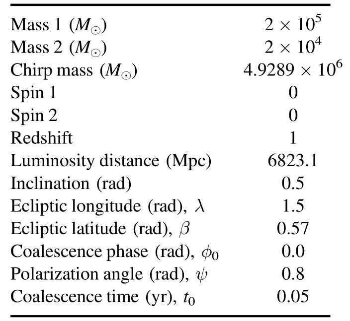
Table 1.The parameter setup of the simulated MBHB merger.The first column shows the parameters and the units for each parameter.

The model is restricted to the quasi-circular and non-precessing system.

At last,we use the dynesty package,a public,opensource,Python package that implements dynamic nested sampling methods for inferring the Bayesian posteriors distribution of parameters and evidence [40].By generating samples in nested “shells”,nested sampling is able to estimate evidence as well as the posterior.And the nested sampling can sample from complex,multi-model distributions.Compared to the Monte-Carlo Markov Chain method,the nested sampling is more suitable to the multi-Gaussian parameter distribution case.Currently,pycbc inference supports the dynesty sample [38].

4.Validation

In this section,we show two test suite results.One example is to show the role of the inclusion of the higher-order harmonics in determining the luminosity distance.The other example is to show the capability of testing GR with LISA constellation.

4.1.Massive black holes signals

To test the performance of LitePIG,we choose a representative MBHB source.The total redshifted mass M=m1+m2=2.2×105M⊙,mass ratio q=m1/m2=10 and the redshift z=1.We can obtain the luminosity distance from redshift by assuming fiducial cosmology with H0=67.1 km s−1Mpc−1and Ωm=1 −ΩΛ=0.32.We set the inclination angle to ι=0.5 and the dimensionless spin parameter,a1=a2=0.All the other parameter values are summarized in table 1.Table 2 shows the optimal SNR,equation(41),of each harmonic for the representative MBHB merger event.When calculating the total SNR,the cross termsbetween modes,can be both positive and negative,causing interference between the harmonics [16].The (3,2)with the(2,2)mode are the two strongly coupled modes.One of the significant influences of the (3,2) mode can affect the amplitude and phase of the (2,2) mode [35].Because of these mode mixing effects,the total SNR shown in the‘total’column will not be the orthogonal sum of each mode[41-44].

Table 2.The optimal SNR from each harmonics.Because of the mode mixing,the total SNR is less than the quadrature of all the harmonics.

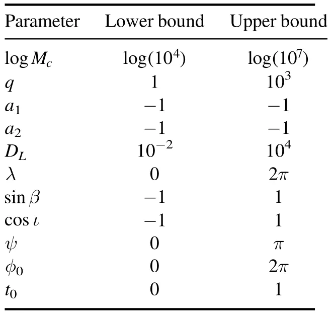
Table 3.The lower and upper bounds of the prior distributions in our Bayesian inference.We assume all priors are uniformly distributed except for the prior on (Mc,ι,β).We assume uniform distributions for isotropically distributed angles on the sphere,so the prior on the inclination angle and ecliptic latitude is uniform distribution oncosι andsinβ.

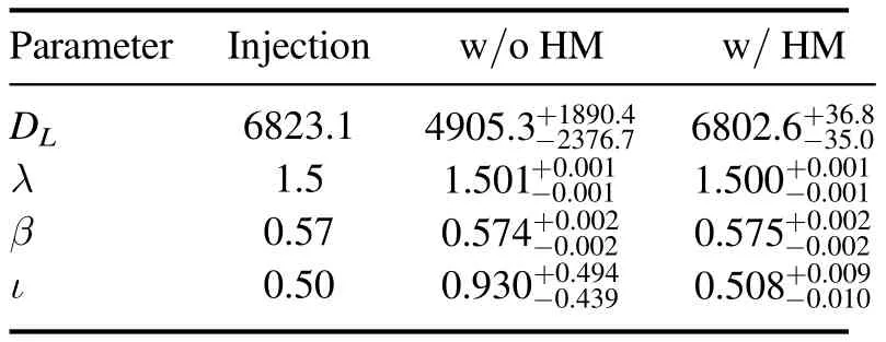
Table 4.The 1σ errors for each parameters.

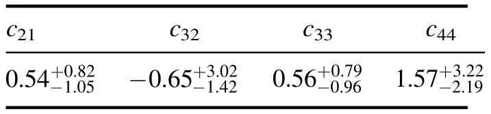
Table 5.2σ deviation from GR of the higher-order harmonic coefficients.

In order to generate the waveform of MBHB,we use pycbc package [38],which currently can only generate the waveform of stellar black-hole binary mergers.Hence,we need to rescale the waveform to obtain our targeted waveform from MBHB.The plus and cross polarization modes of stellar black-hole binary mergers in the frequency domain are assumed to have the following form

where M0is the total mass of stellar black-hole binary.One needs to rescale the frequency and amplitude.Thus,the GW strains of MBHB with total mass M is given by

where the frequency is given by

the amplitude is obtained from

and the phase is idential

By rescaling the waveform,we can generate plus and cross polarization of MBHB for each harmonic.Figure 2 shows the characteristic strain for each harmonic mode.

Figure 5 shows the response for the TDI observables equation (27) in the cases with and without higher-order modes.Though the individual harmonics have fairly smooth amplitude shown in figure 2,the full signal shows obvious wiggles.This is because the frequency dependence of different harmonics is different.

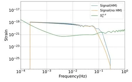
Figure 5.Characteristic strain of full signal compared to the (2,2)dominant mode.The blue curve is the strain of the full signal which is the sum of the individual mode.The orange curve show the strain of the (2,2) dominant mode.The green solid curves show the characteristics strain with the reduced noise PSDf () from equation (25).

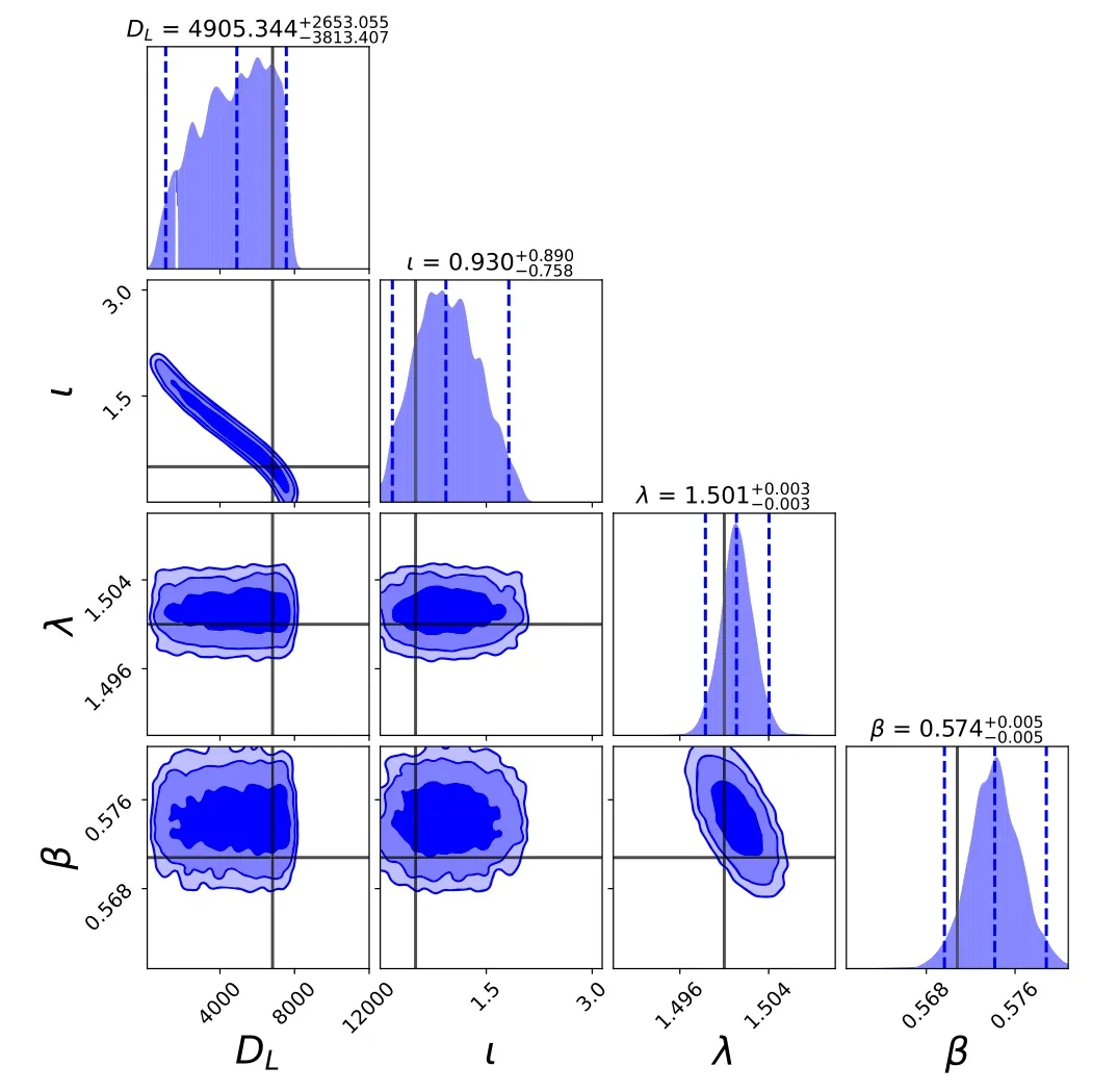
Figure 6.The posterior distribution on the parameters of the MBHB without the higher-order modes.The vertical black lines are the true injectionvalues.The vertical dashed lines show the 2σ credible interval.The posterior distributions show the 1σ,2σ and 3σ contours.

Figure 7.The posterior distribution on the parameters of the MBHB with the higher-order modes.The vertical black lines are the true injection values.The posterior distributions show the 1σ,2σ and 3σ contours.

4.2.Parameter estimation

For the momentum,we do not perform the initial search for the alerted events.Instead,we assume a source has already been identified in the data stream.The priors are given in table 3.The parameter priors for{q,a1,a2,DL,λ,ψ,φ0}are uniform.The log-uniform prior is used on chirp mass.The ι prior is uniform incosιand the β prior is uniform insinβ.We adopt the dynamic nested sampler.In the following analysis,we will present the corner plots of the posterior distribution of the parameters.Figures 6 and 7 show the posterior distribution of the parameters in the cases without and with the higher-order harmonics.The mean and standard deviation can be found in table 4.In the case without the higher-order modes,there is an apparent bias for the parameters in the posterior distribution.The higher-order harmonics can reduce the estimation parameter errors on luminosity distance and inclination angle roughly by a factor of roughly 50.A similar result can be found in table 2 of[45].They find the improvement factor is 10.The difference is because in[45],they choose the mass ratio q=2,and for us,we choose q=10.The role of higher order modes is sensitive to the mass ratio,the higher q is the more important the higher order mode is.As for the mass ratio distribution,one can look at[46],figure 4.As shown in the long-dashed curve(0

During the calculation,it takes about 1 s for each TDI waveform generated.When we estimate four parameters,we run the dynesty package to perform sampling and it takes about 1 h to complete the parameter estimation by parallelizing 50 cores.The parameter sampling points are about 105in total.

4.3.Test GR

The existence of the higher-order modes opens a new window for testing GR.This is because higher-order harmonics carry fruitful information in the ringdown phase of CBC,which corresponds to the strong gravitational field regime.Hence,the test of whether the amplitude of higher-order harmonics is consistent with the predictions of GR delivers a completely new message about the gravitational dynamics close to the black hole horizon.In general,the GW tests of GR can be divided into two categories.The first category is to test the phase evolution.In the second test,one looks for anomalies in the amplitudes of the higher-order modes [47].In our work,we follow [47] and allow for deviation in the amplitudes of the higher-order modes

where the cℓmare the free parameters.In the case of GR,cℓm=0.Sincehℓ,-m=,we have cℓm=cℓ,−m.We use the IMRPhenomXHM template and focus on all modes(ℓ,|m|)=(2,2),(2,1),(3,3),(3,2),(4,4).We simulate the signals generated by MBHB merger and noise according to the LISA setup.The source parameter values are kept the same as in table 1.The only difference is we allow all the cℓmcan vary simultaneously.We assume GR as the fiducial model,so we choose values for the deviation parameter cℓm=0 in the injection.

Figure 8 shows the posterior probability distribution in the GR test.Because the mode amplitudes can vary independently,the inclusion of the higher-order harmonics will not significantly help to break the inclination-distance degeneracy.Hence,one can see that the luminosity distance error in the GR test is much larger than those assuming GR.As for the test of GR,we list the results in table 5.Because of the limitation of data quality,the current GW data detected by LVK can barely give a strict constraint on these parameters[28,48-52].Take GW190412 as an example [28],the posterior on c33is bimodally distributed,due to the degeneracy with the inclination angle.The corresponding errors are almost an order of magnitude worse than here we got.Furthermore,these parameter constraint results are obtained by varying these cℓmone-by-one,not simultaneously as here we did.

Figure 8.The posterior distribution on cℓm for MBMB merger.The vertical black lines are the true injection value.The vertical blue lines indicate 95% confidence intervals.

5.Conclusions

In this paper,we present a new parameter inference system for the gravitational wave data in the millihertz band.We are aiming for the compact binary coalescence originating from the massive black hole binary.In particular,we highlight the role of higher-order harmonics.We show that by including the first four higher-order modes,the famous distanceinclination degeneracy can be very effectively broken.The corresponding errors on the luminosity distance and inclination angle can be reduced roughly by a factor of roughly 50.Furthermore,we show the capability of testing general relativity by LISA constellation.The superb sensitivity of LISA and the robust GW signals from MBHB allow us to detect the ringdown phase of the compact binary coalescence process with a fairly high signal-to-noise ratio.Hence,it opens a new window to explore the strong gravitational field regime,which is the scale of a few times the black hole event horizon.Our results show that the GW from MBHB can simultaneously constrain four of the higher harmonic amplitudes (deviation from GR) with a 95% confidence level of c21=,c32=-,c33=and c44=,respectively.

The software package incorporates the following features:the GW waveform emitted from the massive black hole binaries,the stationary instrumental Gaussian noise,the higher-order harmonic modes,the full response function from the TDI and the Gaussian likelihood function with the dynamic nested parameter sampler.The resulting code,LitePIG,is based on the widely used waveform generator pycbc,which is currently only suitable for the GW emitted from the stellar-mass black hole.We extended this waveform to the MBHB case by some rescaling law.The LISA instrumental noise is imported from the LISA data challenge working package.All of the libraries,on which LitePIG is based,are mature tools that are widely adopted by the GW community.Hence,we believe LitePIG is a reliable package for GW parameter estimation.The code is publicly available on the repository https://github.com/renjiewang888/LitePIG.git.

Acknowledgments

We thank Zhoujian Cao,Xiaolin Liu and Junjie Zhao for the discussion on the gravitational waveform generation.This work is supported by the National Key R&D Program of China No.2021YFC2203001.

ORCID iDs