ESR-PINNs: Physics-informed neural networks with expansion-shrinkage resampling selection strategies

Jianan Liu(刘佳楠), Qingzhi Hou(侯庆志), Jianguo Wei(魏建国), and Zewei Sun(孙泽玮)

1College of Intelligence and Computing,Tianjin University,Tianjin 300350,China

2State Key Laboratory of Hydraulic Engineering Simulation and Safety,Tianjin University,Tianjin 300350,China

Keywords: physical informed neural networks,resampling,partial differential equation

1.Introduction

In the past decade, the rapid development of electronic circuit technology has led to a tremendous increase in computing power of computers.This has led to deep learning applied to an increasing number of scenarios, playing a vital role in several fields such as computer vision,[1,2]natural language processing,[3,4]and speech.[5,6]The neural network is essentially a nonlinear function approximator that automatically extracts its own features by“learning”the data through its powerful fitting ability.This enables a switch from extracting features through feature engineering to automatic feature extraction through date training,thus avoiding human interference as much as possible and realizing the process from“data”to“representation”.

In recent years, along with the wave of deep learning development, deep learning methods have paid more attention to solving partial differential equations (PDEs),[7–10]among which physics-informed neural networks(PINNs)proposed by Raissiet al.[11]have provided a new way of thinking.It constructs a new road to describe the problem,and has successful applications in many areas, such as heat transfer,[12]thrombus material properties,[13]nano-optics,[14]fluid mechanics,[15,16]and vascular simulation.[17]As shown in Ref.[18], PINNs can be used in development of highperformance laser spot center of mass parameter measurement equipment.It transforms the PDEs problem into an optimization problem by using the automatic differentiation mechanism of neural networks to calculate the partial derivatives in the PDEs.The learning process of PINNs is different from that of neural networks applied in other fields,although there are no related studies qualitatively discussing this issue.In other tasks, neural networks learn information about the features of labeled data, while in PINNs the neural network is only constrained by initial and boundary conditions, and the residuals are minimized at all training points in the training process.Unlike the traditional grid methods,the values at all grid points are derived from the transfer of the grid calculation.A PINN can be essentially taken as a complex nonlinear function.PINNs are trained with various conditions as constraints, with the training goal of minimizing the total loss of all training points.The network pays equal attention to all training points during the training process, which leads to a possible propagation failure as mentioned in Ref.[19].The propagation failure phenomenon can be described such that some points in the whole spatio-temporal domain are difficult to be trained and they cause the errors of other points to be larger.This leads the surrounding training points to have difficulty in learning the correct values.This is equivalent to a particular solution of the PDEs learned by PINNs.Although the loss values are small, the solution space obtained is completely different from the correct one.

The PINNs have been improved in many ways, and in Ref.[20] the importance of training points is reconsidered.The allocation points are resampled proportionally according to the loss function,and the training is accelerated by segmental constant approximation of the loss function.In Ref.[19]an evolutionary sampling (Evo) method was proposed in order to avoid the propagation failure problem.This method allows the training points to gradually cluster in the region with high PDEs residuals.The PDEs residual here usually refers to the error between the approximate solution of PINNs and the real solution.Since PDEs, boundary conditions, and initial conditions often differ in numerical values by orders of magnitude, this leads to an unbalanced contribution to each part when the network parameters are updated.The relative loss balancing with random lookback(ReLoBRaLo)was proposed in Ref.[21], aiming to balance the degree of contribution of multiple loss functions and their gradients and to improve the imbalance arising from the training process of some loss functions with large gradient values.Based on an adaptive learning rate annealing algorithm, a simple solution was proposed in Ref.[22].By balancing the interaction between data fitting and regularization, the instability problem due to unbalanced back propagation gradient distribution was improved when the gradient descent method was used for model training.A deep hybrid residual method for solving higher order PDEs was proposed in Ref.[23],where the given PDEs were rewritten as a first order system and the higher order derivatives were approximated in the form of unknown functions.The residual sum of equations in the sense of least squares was used as the loss function to achieve an approximated solution.In Refs.[24,25], the authors paid attention to the importance of the training points.During the training process,the weight coefficients of the training points were adaptively adjusted.Training points with large errors have higher coefficients, leading them to have a larger effect on the network parameters.For time-dependent problems, the authors of Refs.[26,27] firstly trained the network in a short period of time,and then gradually expanded the training interval according to certain rules to cover the whole spatio-temporal domain.This type of method mainly reflects the transfer process of initial and boundary conditions.In Ref.[28],the interaction between different terms in the loss function was balanced by the gradient statistics, and a gradient-optimized physical information neural network(GOPINNs)was proposed,which is more robust to suppress gradient fluctuation.

To show the problem of propagation failure during training in PINNs,an expansion-shrinkage resampling(ESR)strategy was proposed and applied to the PINNs,which is referred to as ESR-PINNs.As introduced above,the PINNs will have the problem of propagation failure during training,but it is often irrational to focus only on training points with large errors.On the one hand,the proposed expansion-shrinkage point selection strategy avoids the difficulty of the network in jumping out of the local optimum due to excessive focus on points with large errors.On the other hand,the reselected points are more uniform reflecting the idea of transmit.Inspired by the idea of functional limit,the concept of continuity of PINNs during training is proposed for the first time.In this way, the propagation failure problem is alleviated and the learning ability of PINNs is improved.In addition,the additional resampling process consumes a negligible amount of time.For a total of 10000 test points,the entire resampling process on the Intel(R)Xeon(R)Silver 4210 CPU@2.20 GHz takes about 20 s in total,with the time mainly cost in the sorting process.

This paper is structured as follows.In Section 2, we describe the PINNs and introduce our method to show how to implement the expansion-shrinkage point selection strategy.In Section 3, we demonstrate our method through a series of numerical experiments.Conclusions are drawn in Section 4.

2.Methodology

In this section, the PINNs are firstly reviewed, followed by a description of the proposed point allocation and selection approach with pertinent details.

2.1.Physics-informed neural networks

Consider the following partial differential equation(PDE)under the initial and boundary condition:

whereu(x,t)represents a field variable associated with timetand spacex,Ndenotes the nonlinear operator,Ωis the spatial domain, and∂Ωis its the boundary, andut(x,t) represents the partial derivative ofu(x,t)with respect to timet.The loss function in PDEs with time terms is often defined as their residual in the form of minimum mean square errors:

whereλ1,λ2, andλ3represent the weight coefficients for the PDE, initial condition and boundary condition, respectively.They are generally given empirically in advance when adaptive weight coefficients are not utilized.For PINNs systems,time and space in PDEs are homogeneous.The fundamental concept is the propagation of the solution into the spatiotemporal domain with initial and boundary values,making the training points satisfy the PDE in the domain.The loss function is used to measure how well the network fits the PDE.In this way, PDEs are solved for their intended purpose.The three terms in Eq.(4)describe how well the network’s output fulfills the PDEs,initial condition,and boundary condition.

2.2.Resampling

With fixed locations of training points for the boundary and initial conditions, the training of PINNs will be significantly influenced by the distribution of training points over the spatio-temporal domain.For instance,increasing the number of training points tends to produce more accurate results for the majority of algorithms.However,due to the limitation of computational resources and computational time,it is often impossible to conduct experiments with large distribution of training points.Therefore,a suitable set of sampling points is important for obtaining accurate solutions.Usually,a random probability distribution,such as LHS and Sober,is chosen for initialization.For different PDEs, the real solution distribution has a certain trend,but the training points with this trend are difficult to be generated by random initialization.Therefore, adaptive resampling is essential for training PINNs of some PDEs as opposed to using preset training points for each iteration.In particular, for some PDEs with drastic changes in time and space, the local values are largely different from other regions, and more points are needed to cope with the rapidly changing peaks.It is essential to dynamically modify the location of particular training points as the training process progresses in order to improve the accuracy of the neural network.In this study, we provide a new method for choosing and allocating points that can enhance the network’s PDEs fitting ability without modifying its structure, parameters and total number of training point.Figure 1 illustrates the structure of the ESR-PINNs.

Fig.1.ESR-PINNs structure.

2.2.1.Point selection strategy

In the vast majority of machine learning problems,the labels of the training data are often given.Even though there are a few mislabels, it is guaranteed that the majority of the data could have accurate labels for training supervision.In contrast,boundary and initial conditions are frequently the driving forces for PINNs training.These conditions control the neural network and spread them to propagate into the interior of the spatio-temporal domain.Random training points usually produce better learning results during propagation in smooth changing regions.Nevertheless,some PDEs have regions with sharp changes, for which randomly initialized training points may not always be able to configure more training points in the sharply changing regions.Thus the solution cannot be reasonably learned by PINNs.Luet al.[29]proposed the first adaptive non-uniform sampling for PINNs, i.e., the residualbased adaptive refinement (RAR) method.This method can be used to calculate the residuals of PDEs by randomly generating far more test points than the training points, and we can select the test points with large residuals as new training points to be added to the original data.Changes to the training point distribution increase the neural network’s accuracy.However, adding only a few test points with large residuals to the training set is undesirable.In our experiments,we find that the distribution of training points may become pathological if the residuals are added continuously in a small region.This pathology is defined as the aggregation of a large number of training points in a small spatio-temporal domain.This pathological distribution may cause PINNs to be difficult to train and thus affects the overall performance.This work introduces a novel computational method for point resampling.As mentioned above,the real challenge for PINNs is that some training points locate in the spatio-temporal domain where the values vary drastically.Since only little training has been carried out,the neural network tends to learn poorly at these locations or gets stuck in local optima hardly jumping out.The set of parameters used in neural networks is intended to reduce the error across all training points.However,when the enormous number of training points that can be more precisely learnt is averaged,the loss values offered by these challenging training points become negligible,and PINNs become unable to depart from the local optimum.As a result,it is necessary to alter the distribution of training points to depart the network from the local optimum.

Table 1.Terminology explanation.

Some of the terminology explanations in the algorithm are listed in Table 1.Firstly, a part of fixed training points is generated according to certain probability distribution as the training point set.Then a large number of fixed invariant data points are generated uniformly in the spatio-temporal domain as the test point set.The calculation of the score in the point selection process is carried out with

whereiindicates the number of iteration andLambis a hyperparameter that controls the ratio between the selection of large residuals and large change points.In the first iteration, i.e.,i=1, only some test points with large residuals are selected as alternative points since there is no reference values.The PDEs residual values of all test points are recorded as res1at this time.The selected alternative points enter into the point generation part, in which the new generated training points will be added to the fixed training point set for the first iteration.The residual values of all test points before this iteration are recorded as resold.Wheni／=1, the PDEs residual values of all test points will be recalculated as resi,and according to Eq.(5),the score is calculated,and its value represents the ranking of this point in the test points.The higher value of the corresponding part ofLamb,with unchanged test point,indicates that the neural network was not sufficiently optimized for this point in the previous iteration to make its output more compatible with the PDEs.If this item has a value larger than 1, the neural network works poorly at this test point as a result of the negative optimization in the previous iteration.This avoids to some extent that only the points with the largest residuals are considered in the point selection process,while a large number of training points with moderate residuals are ignored.This can lead to a reduction in the importance of these points during the training process, which may result in these points never being effectively optimized.Note that the ranking of this point’s PDEs residual among those of all other points replaces the value of res in this work,and the first component is expressed as the ranking of the position among all ratios.By using Eq.(5), the output score of Eq.(5)is taken as the final ranking, and the score inaccuracies brought by the difference in order of magnitude between the two portions are prevented.

2.2.2.Training points generation method with expansion-shrinkage strategy

To locate decent training points,the selection of points are carried out in the steps described above,and the generation of enlarged alternative points is performed in this section.

Table 2.Parameter explanation.

Table 2 describes the meaning of the parameters.The topmipoints are discovered by sorting the scores after they have been computed in the above section (we select one third to one half of the total number of test points).These locations are then used as the center of a circle with a diameter of ∆x(since the fixed test point interval in the algorithm is ∆x, the radius here is set to ∆x/2 in order to reduce the impact on other test points)to produce new randomly generatednialternative points(niis often between 2 and 10).This is equivalent to an expansion of the alternative points generated in the part of the algorithm to obtainnitimes more alternative points.At this time, the residuals of the PDEs of the newly generated alternative points are calculated, and the largestmi+1points are taken as the alternative points in the next round.The remainingmini −mi+1expansion pointsPiare further randomly chosen as training points to be saved.The current operation is then repeated with the chosenmi+1alternative points.Them4points with the greatest residuals from the final round of generated alternative points are added to the training set after this operation is repeated three times to produce a total ofP1+P2+P3training points,along with them4points.Figure 3 depicts this process.

Fig.3.Training points generation method with expansion-shrinkage strategy process.

We call this operation as the expansion-shrinkage strategy,and after obtaining the alternative points through the first part of the algorithm, we first perform expansion around the alternative points.Note that the expansion process does not include the alternative points themselves, and we choose to generate random points in a small field of alternative points to replace them.This is carried out to prevent that some data points are inherently difficult to train from being chosen more than once during numerous cycles.The distribution of training points as a whole is then destroyed and turns pathological, making it a challenge to train points under such a distribution.This is because PINNs cannot supervise the training points in the spatio-temporal domain during training.The proposed method of randomly creating new points around alternative points as replacement points improves the continuity in this neighborhood.We use the concept of function limits in this context, i.e., arbitraryε>0 and presenceδ>0.When|x−x0|<δ, we have|f(x)−f(x0)|<ε.Sufficiently minor perturbationsδto the input values have a relatively modest effect on the final output.As each layer’s weight coefficients are constant when the network is propagated forward, the output changes caused by input perturbations are minimal.Therefore,by boosting the continuity within a specific band of big residuals, we attempt to ameliorate the subpar training outcomes caused by the propagation problem.

After obtaining a total ofminipoints withnitimes of expansion, the contraction process is entered.First, themi+1points with the largest residuals are selected as alternative points for the next expansion, and thenmi+1points are randomly selected as training points among the alternative points.Due to the random point selection, the obtained selection points are more uniform.The purpose is to avoid excessive focus on high residual points in the process of generating the training points.In the algorithm, we can divideP1+P2+P3into several times for selection similar to a mountain peak,of which the summit indicates the area with high residuals where the majority of training points are placed, and consequently the density of training points increases as the peak tightens higher.In order to make the process transition more gradually and prevent all the train points from condensing in a small area as much as possible,alternative points in the contraction process are also taken into consideration.In addition to paying attention to the high residual points, the medium residual points also receive more attention.The distribution of training points is made more appropriate for PDEs and this portion of the points is ensured to receive more attention during the training process.It is equivalent to homogenize all the high residuals if only a few points with the greatest PDEs residuals are chosen as training points, which does not accurately reflect the significance of various training point locations.It is illogical to consider all large residuals homogeneously because residuals frequently change greatly during the training of PINNs,and this is represented in our algorithm.Additionally, the residual variance of the training points may become flatter as a result of random selection of the alternative points in the expansion process,which is an advantage in the training of ESR-PINNs.

3.Results and discussion

In this section,we present several numerical experiments to verify the effectiveness of the proposed ESR-PINNs.

3.1.Burgers equation

The Burgers equation is a nonlinear PDE that models the propagation and reflection of shock waves.It is a fundamental equation used in various fields such as fluid mechanics, nonlinear acoustics,and gas dynamics.Here we can write it as

Our experiments revolve around the forward problem, where the parametersa1anda2are 1.0 and 1/100×π,respectively,and the mean square error is used as the loss function.

The following settings are selected for PINNs.Using Sober for random point selection, with a total of 80 points on the boundary and 160 randomly selected training points as the initial conditions, for a total of 2540 training points in the spatio-temporal domain.The neural network structure has three layers with 20 neurons in each layer.Three iterations of point selection,with 80 points are set on the boundary,160 points for the initial condition,and 1000 fixed points generated randomly by Sober as the training points.

Table 3.Parameter setting for the Burgers equations.

Table 3 shows the parameter settings.Each iteration is trained for 10000 epochs.During the first expansion, we setm1=2500 andn1=4, and then 10000 expansion points are obtained.Next, the residuals of PDEs for all extended points are calculated, and thenm2= 2500 points with the largest residuals are selected as alternative points for the next round.Among the remaining training points, a total ofP1= 300 points are randomly selected as the first extended training points using Monte Carlo method.We use the following parameters in the second and third round of iterations:n2=4,m3=2000,P2=300,n3=5,P3=400 andm4=500.After three rounds of expansion and contraction operation, a total of 1500 retention points are selected as new training points added to the training set.First, we use the Adam optimizer for initial training of the neural network with 10000 epochs at a learning rate of lr=1×10−3, followed by the L-BFGS optimizer to finely tune the neural network with a total of 10000 epochs.Without using any early stopping strategy and dynamic weighting algorithm, the weighting coefficientsλi(i=1,2,3)in Eq.(4)are taken as 1.

Figure 4 shows the ESR-PINNs solution compared with that of the original PINNs.It is obvious that ESR-PINNs significantly reduce the absolute errors.By looking at the error distribution of PINNs as shown in Fig.4(d), it can be seen that there is indeed some dissemination failure problem.This problem is somewhat improved by changing the distribution of training points in ESR-PINNs.The overall error is reduced by about one order of magnitude.In Table 4 theL2errors of the ESR-PINNs and original PINNs for differentLambare shown.It can be seen that theL2errors of ESR-PINNs are significantly smaller than that of the original PINNs for anyLamb.The algorithm achieves the best performance forLamb=0.4.

Fig.4.Numerical solutions of(a)PINNs and(b)ESR-PINNs,and absolute errors of(c)PINNs and(d)ESR-PINNs for the Burgers equation.

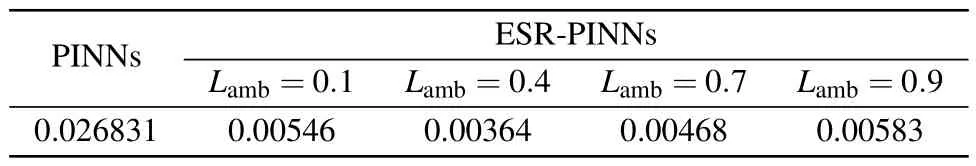
Table 4.Comparison of L2 errors for the Burgers equation: PINNs and ESR-PINNs with different Lamb.

Figure 5 shows the comparison of the losses of PINNs and ESR-PINNs with differentLambduring the training process.It can be seen that during the pre-training phase,all experimental groups converge to a fairly low loss, but the optimal solution is not obtained at this time.As the training proceeds,the loss of PINNs does not change much, but the neural network at every point is finely tuned to make the PINNs output more consistent with the PDEs.In the experimental group of ESRPINNs, it can be seen that loss changes dramatically as the algorithm takes different training points.With each iteration of reselected points, the loss tends to rise and then falls, and it is always higher than that of the original PINNs.The loss of the original PINNs is almost constant after 20000 training epochs.However,theL2error of PINNs at the end of training is large,which indicates that the neural network falls into a local optimum during training.The original PINNs have limited ability to jump out of the local optimum, resulting in disappointing outcomes.The distribution of training points has a significant impact on the performance of the original PINNs and extremely worse results most probably appear (the loss function stays at 1×10−3and is difficult to be optimized).The expansion-shrinkage strategy of ESR-PINNs selects the hardly optimized points with large errors as extra training points,aiming at reducing the total error in the training process by decreasing the errors of them.However,adding these points with high residual to the training set will naturally lead to higher loss function values.This is the reason why the loss function of PINNs is lower than that of ESR-PINNs for some PDEs.These “tough” points have a great impact on the PINNs results,so finding and optimizing them appropriately will allow the other training points to be better optimized and therefore significantly reduce theL2error.By dynamically adjusting the distribution of training points while maintaining some training points unchanged, the stability of the neural network training can be improved as the point selection iteration goes on.The placement of training points reduces the pathology issue that arises in neural networks and improves the numerical precision.However, the experimental findings with loss function fluctuation demonstrates that there is no direct relationship between the numerical accuracy and the loss function values.A low loss may correspond to a large error.

Fig.5.The losses of PINNs and ESR-PINNs with different Lamb for the Burgers equation.

3.2.Allen–Cahn equation

Next,the Allen–Cahn equation is studied because it is an important second-order elliptic PDE.It is a classical nonlinear equation originated from the study of phase transformation of alloys,and it has a very wide range of applications in practical problems such as image processing,[30]and mean curvature motion.[31]It can be written as

where the diffusion coefficientDis 0.001 and theL2norm is used as a measure.As a control, we select the PINNs setup as follows: using Sober for random point selection, with 400 points on the boundary,800 for the initial condition,and 8000 training points in the spatio-temporal domain.The neural network structure has three layers with 20 neurons in each layer.In order to improve the convergence speed and accuracy, the initial and boundary conditions are hard-constraints in the experimental setup.[32]

Table 5.Parameters set for the Allen–Cahn equation.

Table 5 shows the parameter settings.The ESR-PINNs method is set up for a total of three iterations.The boundary and initial condition points are set as PINNs, and 5000 fixed training points are randomly generated.After three rounds of expansion and contraction,a total of 3000 retention points are selected and added to the training set as new training points.Other settings are the same as those for the Burgers equation,but the total training number is 40000.

Table 6.Comparison of L2 errors for the Allen–Cahn equation: PINNs and ESR-PINNs with different Lamb.

Figure 6 shows the ESR-PINNs solution compared with that of the original PINNs.In Table 6,theL2errors of the original PINNs and ESR-PINNs with differentLambare shown.In the course of experiments,we found that the best and most stable results are obtained whenLamb=0.4.The experimental results show a relatively large variance atLamb=0.9.When the effect is poor theL2errors will be similar to that of the original PINN.However,when the selected point is exciting,L2errors will drop to about 0.002.This may be due to the fact that whenLambis relatively large, the algorithm pays more attention to the selection of training points with poor optimization effect in the iterative process.That is,those training points locate in the domain where the residual value changes less before and after this training.The locations with large PDEs residuals in the experiment are always concentrated in a small area.Neural networks tend to be more sensitive to low-frequency data during training,[33]and the vast majority of regions have small residuals.This results in these training points being difficult to be optimized.In ESR-PINNs,especially whenLambis relatively small, the algorithm takes this part of training points into full consideration.ESR-PINNs are actually optimized for the training process,i.e.,optimization from focusing on large error areas to the overall situation as much as possible.The overall error reduction is achieved by bringing down the error in more areas with moderate error.

Fig.6.Numerical solutions of (a) PINNs and (b) ESR-PINNs, and absolute errors of (c) PINNs and (d) ESR-PINNs for the Allen–Cahn equation.

Fig.7.The losses of PINNs and ESR-PINNs with different Lamb for the Allen–Cahn equation.

Figure 7 shows the loss values of the original PINNs compared with those of ESR-PINNs with differentLambduring the training process.The loss curve forLamb= 0.4 shows that even if the results obtained in the pre-training phase are not satisfactory,ESR-PINNs can still improve the experimental accuracy by dynamic point selection.That is, because the training proceeds,the loss of the experimental group with bad performance in the early period can also be reduced to about the same value as the normal experimental group.The ESRPINNs better balance the large error points and small variation points,which is probably the reason for the best and stable results whenLambis 0.4(see Table 6).

3.3.Lid-driven cavity

The lid-driven cavity, a classical problem in computational fluid dynamics, is chosen as the object of study for the last experiment.This problem is chosen to verify the performance of the method for a time-independent problem, and to confirm that ESR-PINNs can maintain training points in the moderate error region and converge in the large error region.As a steady flow problem in a two-dimensional cavity, it is governed by the incompressible Navier–Stokes equations, in dimensionless form,as

whereurepresents the velocity field andprepresents the pressure field.The Reynolds numberRe=100 is chosen in the experiment.The high-resolution dataset generated using the finite difference method is used as the evaluation criterion,where

We select the PINNs setup as follows:using the LHS distribution for random point selection, with 400 points on the boundary,and 3000 training points in the spatio-temporal domain.The neural network structure has five layers with 30 neurons in each layer.

In the lid-driven cavity experiment, the ESR-PINNs method is set up for a total of two iterations.We randomly select 400 points on the boundary, and the LHS is applied to randomly generate 2000 fixed training points.Each iteration is trained 10000 epochs,Table 7 shows the parameter settings.Other settings are the same as the Burgers equation, but the total training number is 40000.

Table 7.Parameter setting for the lid-driven cavity.

Figure 8 shows the ESR-PINNs solution compared with the high precision solution obtained by the grid method.[34]In Table 8 theL2errors of the ESR-PINNs and PINNs with differentLambare given.The best results are obtained for ESRPINNs whenLamb=0.4.In the experimental results, the errors are mainly concentrated at the top left and top right corner points.The reason is that singularity problem arises at the two corner points.That is,the velocity at the top cap is 1 and the velocity at the left and right walls is 0.The values at the points (0, 1) and (1, 1) create an ambiguity.Figure 9(a)shows the results after the first round of iterative expansion,and Fig.9(b)presents the results after three rounds of expansion and shrinkage.Compared with Fig.9(a),the distribution of training points in Fig.9(b)not only adds new training points in all high-error areas, but also gathers high-error points in high-error areas together,and the aggregation process of training points is generally smooth.

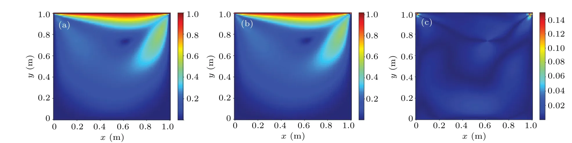
Fig.8.Flow in the lid-driven cavity: (a) reference solution using a finite difference solver, (b) prediction of ESR-PINNs, and (c) absolute point-wise errors.

Table 8.Comparison of L2 errors for the lid-driven cavity: PINNs and ESR-PINNs under different Lamb.

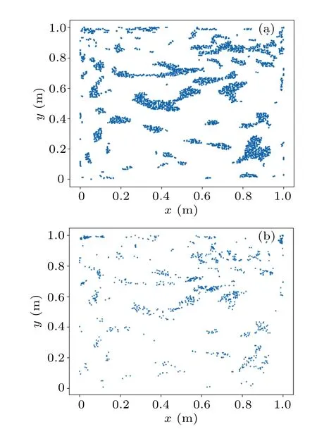
Fig.9.Distribution of training points(a)at the end of the first expansion and(b)at the end of the resampling algorithm.

Figure 10 compares the loss values for the original PINNs and ESR-PINNs under variousLambconditions throughout training.All experimental groups converge to a smaller loss once more during the pre-training phase.The original PINNs’convergence slows down as the number of training instances rises.The loss values of ESR-PINNs are higher than those of the original PINNs because some high residuals are selected and added to the training set, but the overall performance is better than that of the original PINNs.The loss values of ESRPINNs with changing selected points are similar to those in the previous experiments, but the average performance is better than that of PINNs.

Fig.10.The losses of PINNs and ESR-PINNs with different Lamb for the liddriven cavity problem.

4.Conclusions

In this study,we reevaluate how training points influence PINNs performance.Due to the distribution of training points,the original PINNs may be challenging because the training points are invariant during the training process.In experiments, this issue comes up frequently.A poor training point distribution may result in the PINNs entering an impossibleto-exit local optimum, and hence producing an undesirable solution.PINNs may also fall into a certain PDEs solution because of a poor distribution.The difference between the PINNs solution and the correct solution is still large, even though the loss may be small at this point.The ESR-PINNs are developed as a solution to this issue.

In ESR-PINNs, the resampling process is added to the training process of PINNs.The whole resampling process is divided into two parts, and the first one is point selection.We propose for the first time that the point selection process should not only focus on the training points with large errors,but also consider the parts that are not optimized during the iterative process.In the second part, we are inspired by the function continuity not only to place more training points in high error regions,but also to make the aggregation process of training points smoother.Thus,we avoid the problem that the network crashes due to a large number of training points in a small region.Then we verify the effectiveness of ESR-PINNs through three experiments, which prove that ESR-PINNs can effectively improve the accuracy of PINNs.

At present, our study is relatively limited, and some aspects cannot be answered accurately, e.g., how to determine the fixed number of training points and the proportion of resampling parts,and how many rounds of expansion-shrinkage process are appropriate.In addition, this method can be inserted into PINNs as a plug-and-play tool,but the specific parameters need to be set in conjunction with PDEs.

Acknowledgements

Project supported by the National Key Research and Development Program of China(Grant No.2020YFC1807905),the National Natural Science Foundation of China (Grant Nos.52079090 and U20A20316),and the Basic Research Program of Qinghai Province(Grant No.2022-ZJ-704).