Evaluation of Different Cloud Microphysics Schemes on the Meteorological Condition Prediction of Aircraft Icing

，，，，，

1.Engineering Techniques Training Center，Civil Aviation Flight University of China，Guanghan 618307，P.R.China；

2.School of Aeronautics，Northwestern Polytechnical University，Xi’an 710072，P.R.China；

3.China Academy of Aerospace Aerodynamics，Beijing 100074，P.R.China

Abstract: Flight safety is at risk due to complex icing meteorological conditions，highlighting the need for accurate prediction models that integrate geographical features.The mesoscale weather research and forecasting（WRF）model is utilized to simulate two icing events on Mt.Washington in the United States with four cloud microphysics configurations.Results indicate that the predicted liquid water content（LWC）and temperature are well matching results in the existing literature，and the Morrison configuration provides the most significant performance in the error analysis.Additionally，the sensitivity of horizontal resolution and cloud microphysics scheme for LWC and the mean effective diameter of cloud droplet（MVD）prediction is discussed，with higher horizontal resolution demonstrating greater accurate performance due to terrain-induced vertical motions.The study concludes with an analysis of icing intensity using the IC index，showing pronounced spatiotemporal variability and sensitivity to cloud microphysics schemes.Overall，this work enhances our understanding of cloud microphysics schemes and provides a base for selecting appropriate cloud microphysical solutions for icing weather prediction.

Key words：aircraft icing；numerical prediction；cloud microphysics schemes；meteorological environment；weather research and forecasting（WRF）model

0 Introduction

When aircraft fly through high-altitude clouds，supercooled liquid droplets impact the aircraft surface，resulting in icing accretion，which perhaps causes severe aerodynamic and flight mechanical effects［1-2］.Hence，aircraft icing is an essential hazard to flight safety.With the increase in flight density，there were 380 icing-related accidents from 2003 to 2008［3］.Therefore，it is of urgent practical significance to develop reliable methods for predicting the regions of icing risk and its severity.The Federal Aviation Regulations（FAR）Part 25 Appendix C［4］has defined atmospheric icing conditions，stating that aircraft icing mainly depends on the icing meteorological environment，such as the cloud liquid water content（LWC），the mean effective diameter of cloud droplet（MVD），the relative humidity（RH），the ambient air temperature，pressure，and cloud extent，etc［4］.

Icing prediction algorithms are crucial to diagnos is of aircraft icing conditions.Over the years，various algorithms have been developed based on evolutionary forecasts and calculations of parameters related to icing.The first icing algorithm，developed by Schultz et al.［5］，used temperature and RH to predict icing probability with thresholds derived from pilot reports.The National Center for Atmospheric Research（NCAR）proposed an icing severity index，which considered the atmosphere temperature，LWC，and MVD［6］.Subsequently，three improved icing algorithms，known as T-RH algorithms，were developed by the Research Application Program（RAP），NCAR，and the National Aviation Weather Advisory Unit（NAWAU），respectively，based on combinations of the numerical weather prediction（NWP）model’s temperature，and RH and the vertical thermodynamic structure［7］.The forecast icing potential（FIP）and current icing potential（CIP）techniques，based on decision trees and a fuzzy logic approach，were then introduced by NCAR to integrate various model variables，such as temperature，LWC，RH，and cloud top temperature［8-9］.Subsequently，the improved CIP algorithm was proposed，which combined ground-based observations and sounding data to calculate the climate distributions of icing and supercooled large droplets［9-11］.Overall，these algorithms have significantly contributed to the safety of aviation by enabling pilots to predict and avoid hazardous icing conditions.

However，there are significant differences in the description of distinct cloud microphysics schemes used in NWP models.These differences include the number of particle classifications，densities，distribution spectra，and end-of-fall velocities，as well as the physical description and treatment of specific cloud microphysical processes.Nygaard et al.［12］compared the accuracy of explicit predictions with different cloud microphysics schemes at different horizontal resolutions and discussed how well the MVD can be diagnosed based on the optimal cloud microphysics scheme.Podolskiy et al.［13］conducted a series of quantitative comparisons of various numerical predictions with three different cloud microphysics schemes and concluded that the finer spatial resolution had a more accurate performance.Davis et al.［14］evaluated the icing model’s effects with a combination of nine parameterizations on icing events in the Swedish wind field.Merino et al.［15］used four microphysics and two planetary boundary layer schemes to investigate the capability of the weather research and forecasting（WRF）model to detect regions containing supercooled cloud drops.Diaz-Fernandez et al.［16］evaluated twenty different WRF model configurations in an initial analysis and used the best combination to diagnose the characteristic variables of the mountain wave associated with icing.

Although the aforementioned studies highlight the understanding importance of cloud microphysics schemes on NWP models for atmosphere icing，the effect of different cloud microphysics schemes on the icing severity has not been further evaluated.In this paper，first，two icing events on Mt.Washington in the United State are simulated with four cloud microphysics configurations，and the predicted LWC and temperature are well matching with results from the literature.Second，the sensitivity of horizontal resolution and cloud microphysics scheme for LWC and MVD prediction is discussed.The IC index is employed for the analysis of icing intensity.Third，the spatiotemporal variability of icing severity under simulations with different microphysics schemes is evaluated，and the differences in the corresponding IC index distribution are revealed.Through this work，a better understanding of cloud microphysics schemes can be enhanced，and a basis for selecting appropriate cloud microphysical solutions for icing weather prediction can be provided.

1 Numerical Model Setup

The mesoscale numerical weather prediction model used in this study is the advanced research WRF（ARW）modeling system，version 4.2，which was jointly developed by the National Centers for Environmental Prediction（NCEP）and NCAR，among others.The WRF model is based on a compressible non-hydrostatic dynamical framework and a terrain-following coordinate system.It employs an Arakawa-C type grid to divide the computational domain in the horizontal direction，with multiple grid nesting capabilities and various parameterization schemes for atmospheric physical processes.Combined with global meteorological data and assimilation techniques，the WRF model is widely used in simulating of weather phenomena at air quality modeling，different temporal/spatial scales，atmospheric oceanic and idealized simulations［17］，and it also has excellent performance for icing meteorological analysis［15-16］.

This study intends to analyze and evaluate the sensitivity of cloud microphysics schemes on icing meteorological condition prediction using two threeday cases.The first dataset（Case 1）was from April 1st to 3rd in 2013 and the second（Case 2）from March 10th to 13th in 2011.The Simulations take the geographic location of Mt.Washington（44.267 °N，71.3 °W，1 917 m），the tallest peak in the northwestern United States，as the center point of the simulated area.Initial and boundary conditions are furnished by NCEP reanalysis with 1° horizontal grid spacing resolution and a temporal resolution of 6 h.

Numerical simulations are carried out by three levels of nested domains，with the inner model domain embedded into the outer model domain，to analyze the characteristics in detail that influences the formation of icing conditions，as shown in Fig.1.The horizontal resolutions of the domains are 9，3，and 1 km，and the vertical resolution is set to 27 linear levels.Besides，the real elevation of Mt.Washington is approximately 1 917 m，but the model height in the innermost domain is only 1 656 m，reduced by 261 m.More detailed domain configuration and topography are shown in Table 1.

Fig.1 Schematic diagram of the nested domains

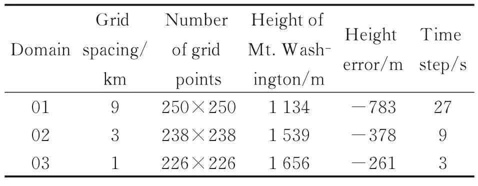
Table 1 Domain configuration and Mt.Washington elevation in the WRF simulations

The selected parameterization schemes include the Dudhia scheme，the Rapid Radiative Transfer Model（RRTM）scheme for shortwave and longwave radiation，and the Yonsei University（YSU）scheme for planetary boundary layer.The MM5 similarity surface layer scheme described by Fairall，and Noah Land Surface Model，are considered.The Kain-Fritsch（K-F）cumulus scheme is employed for nested domains.

To optimize the parameterization schemes，four microphysics schemes that are essential in forecasting various types of hydrometeors，are evaluated：WRF single-moment six-class（WSM6）scheme［18］，Thompson six-class microphysics scheme［19］，Morrison six-class double-moment scheme［20］，and the double-moment Milbrandt-Yau scheme［21］.

The scheme［18］considers the treatment of six types of hydrometeors including rain，water vapor，cloud water，snow，cloud ice，and graupel.This scheme is capable of modeling mixed-phase change processes and supercooled water，and treats the saturation adjustment processes of ice and water separately.It is particularly suitable for grid point studies where the grid distance is between cloud scale and mesoscale.

The Thompson six-class microphysics scheme［19］incorporates prognostic equations for the mass concentration of five hydrometeors：Cloud water，cloud ice，rain，snow，and graupel.It has a great performance in the prediction of LWC，as special attention is paid to the formulation of the snow category.

The Morrison six-class double-moment scheme［20］，based on the full two-moment scheme，predicts the mass concentration of five hydrometeors in consistence with the Thompson scheme，as well as the number concentration of four species：Cloud ice，snow，rain，and graupel.The prediction of both the mass mixing ratio and number concentration of these four water species allows a more robust description of size distributions.

The Milbrandt-Yau scheme［21］is also a full double-moment scheme，which shares many features with the Morrison two-moment scheme.However，one major difference is the calculation of the droplet action.The Milbrandt scheme allows the cloud number concentration to evolve.

Three indicators are employed to evaluate the four microphysics schemes in this work：（1）Mean absolute error（MAE），（2）root mean squared error（RMAE），（3）mean absolute percentage error（MAPE）.The indicator expressions are demonstrated as

whereymeasandypredare the observed and the predicted values，respectively；Nis the quantity of samples.

2 Validation of Numerical Model

2.1 Validation of predicted temperature and LWC

The icing meteorological conditions in the targeted domain is simulated by means of the four microphysics schemes，and the optimal parameterization scheme is determined through error analysis among the four schemes.The comparison between the observed and the predicted values of the temperature at 2 m and LWC at the domain’s center point for Case 1 is demonstrated in Figs.2，3，respectively，from 6：00 on April 1st to 18：00 on April 3rd in 2013，where the black dot represents the observed values，the red line represents the results in Ref.［22］，and the purple，magenta，blue，and olive lines represent the WSM6，Milbrandt，Morrison，and Thompson schemes，respectively.

It is evident that although there are deviations between the predicted values of the four microphysical process schemes and the observed values at certain individual time points，all the four schemes accurately predicted the temporal trends of temperature and LWC in Case 1，consistent with the literature.

The error analysis of temperature and LWC prediction with four microphysics schemes is shown in Table 2.It demonstrates that each parameterization combination has an outstanding performance in temperature and LWC prediction，with a MAE of only about 0.75 ℃ and 0.12 g/m3.The RMSEs for the schemes are less than 0.970 and 0.18，and the MAPEs are less than 0.100 and 0.58，respectively，indicating that all parameterization combinations have sufficient numerical accuracy in temperature and LWC prediction.Continuous time series are depicted in the line graphs in Fig.3，however，the MAE，RMSE，and MAPE values are only based on the sporadic times when there are measurements available in the literature.In particular，the MAE，RMSE and MAPE of LWC in the literature are 0.116 g/m3，0.146，and 0.478，respectively，whereas the corresponding errors of the prediction with the Morrison scheme are only 0.120 g/m3，0.146，and 0.470.

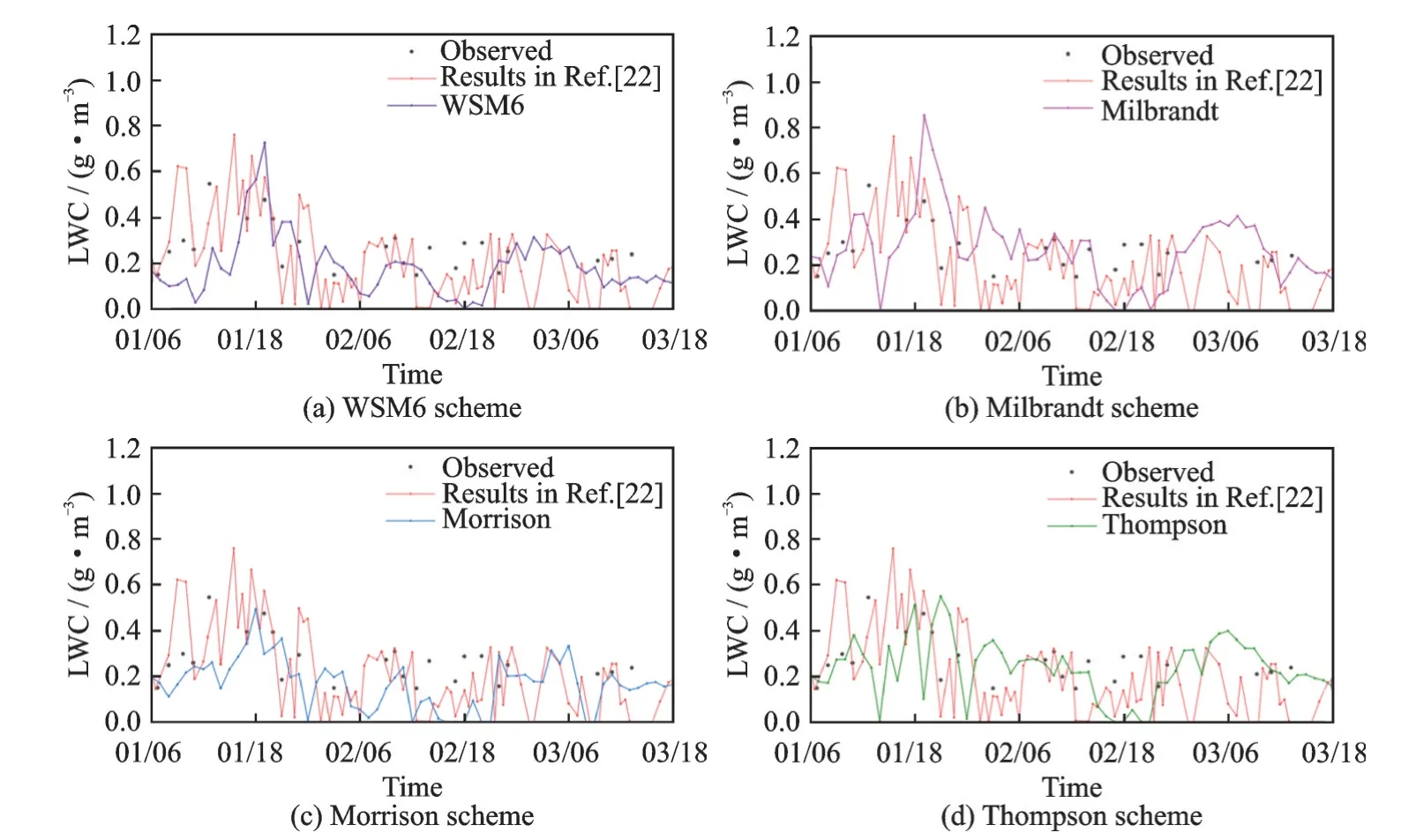
Fig.3 Comparison of LWC in different microphysics schemes in Case 1

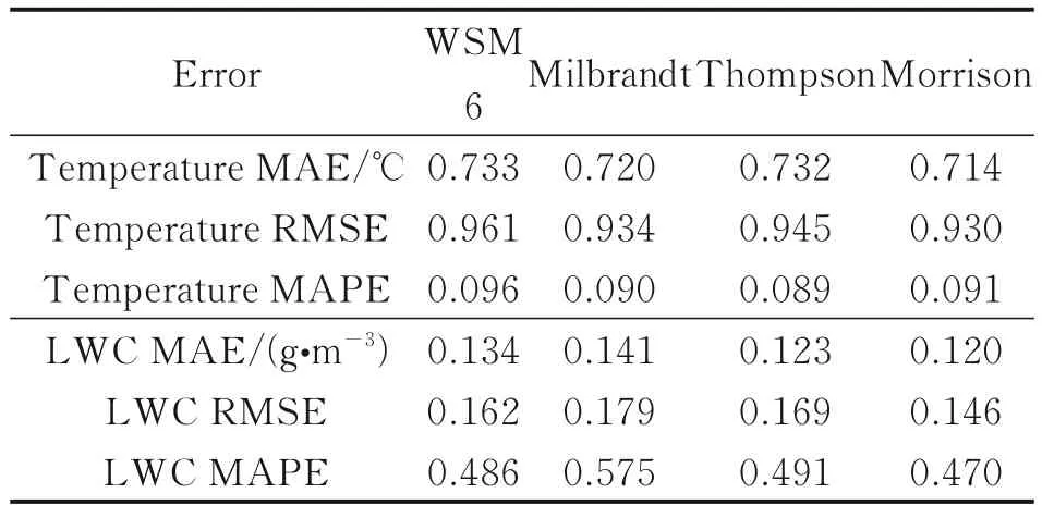
Table 2 Error analysis of temperature and LWC prediction

As shown in Fig.4，there is a general improvement in MAE when increasing the resolution，as the finer horizontal resolution allows better prediction of cloud water due to terrain-induced vertical motions.Meanwhile，the choice of microphysics scheme is also verified to be quite sensitive in Fig.4.The Morrison microphysics scheme results in the best match between observations and simulations，with an MAE of 0.120 g/m3，compared to 0.123，0.134 and 0.141 g/m3for the Thompson，WSM6，and Milbrandt schemes，respectively.

Fig.4 MAE of predicted LWC for simulations with various cloud microphysics schemes

2.2 Prediction of MVD

The particle spectra of hydrometeors can be described by different functions，resulting in major differences in the particle distribution and the treatment of particle spectral parameters.Observational studies show that the Gamma function can better describe the particle spectrum of hydrometeors in clouds［23］.A generalized gamma distribution for the cloud liquid water can be described as follow［19］

whereN(D) is the number of droplets per unit volume；N0the intercept parameter；andDthe particle diameter.μandλare the size distribution shape parameter and the slope parameter，respectively，given bywhereNcis the droplet concentration given as droplets per cubic centimeter；ρwthe density of water；andΓ( ) the gamma function.

By solving the above equations，a diagnostic of MVD can be obtained［24］

Based on the droplet concentration and the assumed size distribution，characteristic droplet sizes can be diagnosed，such as MVD，which is one of the largest uncertainties in the prediction of atmospheric icing.Among the four cloud microphysics schemes used，the Morrison and Thompson schemes apply only a fixed droplet number concentration，which is respectively set to 250 and 100 per cubic centimeter by default throughout the simulations［12，22］.The Milbrandt configuration，on the other hand，could obtain the droplet concentration as output variables，while the WSM6 scheme cannot directly forecast the number concentration.Comparing the predicted MVD at the domain’s center point with the observed values from the literature，Fig.5 shows the results for simulations with the Morrison，Thompson，and Milbrandt microphysics schemes.Although some data points for these configurations are lost in the innermost model domain due to the lack of clouds，it is enough to evaluate three microphysics schemes.The simulations exhibit a systematic high bias，especially in results from Ref.［22］and the predictions by the Thompson scheme.

Fig.5 Comparison of MVD with three different microphysics schemes in Case 1

Fig.6 shows that predicted versus observed MVD using the above-mentioned three microphysics scheme.Compared to the Morrison configuration，MVD is more overestimated when the Thompson scheme is adapted.MAEs of the predicted MVD of three microphysics schemes are 4.131，5.786，and 4.493 μm，respectively，and the Morrison scheme also achieves the best performance among three schemes，with RMSE and MAPE of 4.690 and 0.346，respectively.It demonstrates that the Morrison scheme is capable of capturing the evolution of MVD changes more accurately.

Fig.6 Predicted versus observed MVD using the Morrison,Thompson and Milbrandt microphysics schemes

3 Analysis of Aircraft Icing Intensity

The IC index recommended by International Civil Aviation Organization（ICAO），is employed to diagnose the icing severity in this study.The IC index as an initial diagnostic algorithm indeed has many drawbacks，such as ignoring the role of vertical thermodynamic structure and liquid water content，and generally overestimating the extent of icing areas，even indicating it in cloud-free areas.However，the IC index also has the advantages of being a simple diagnostic algorithm with high detection probability.Compared to others algorithm，the IC index can quickly diagnose the icing intensity.Thus，it is a good exploration to evaluate the sensitivity of micro-physical schemes to icing environment prediction using the IC index.Studies indicate that aircraft are most susceptible to ice accretion when flying in a temperature ranging from 0 ℃ to-14 ℃ or encountering large supercooled water droplets.The most severe ice accretion typically occurs between -5 ℃ and -9 ℃.The IC index can be determined based on the temperature and humidity range where ice is likely to accumulate［25-26］

where RH is relative humidity with the unit of %，andtthe temperature with the unit of ℃.In Eq.（8），RH is used to linearly match the growth process of the number and size of water droplets in clouds，and the quadratic of temperature is utilized to fit the growth of water droplets.When RH is less than 50% ortexceeds the range from 0 ℃ to -14 ℃，the droplet growth rate is assumed to be 0，and no ice accretion is considered to occur.

According to FAR Part 25 Appendix C［4］，aircraft icing is primarily influenced by meteorological factors and flight status.Predicting the icing meteorological environments based on the WRF model can obtain the spatiotemporal distributions of meteorological parameters，such as atmospheric temperature，air pressure，LWC，and MVD.Furthermore，the IC index in the target region can be calculated based on Eq.（8）.Specified configurations of the WRF model are discussed in Section 1.

The predicted IC index from the Morrison configuration in Case 1 is taken as an example，and Figs.7，8 exhibit the IC index contours of altitude layerη=6 at different times on April 1st and of altitude layerη=6，10，14 at 06：00 on April 1st.Figs.7，8 demonstrate that the IC index varies significantly with both time and elevation.

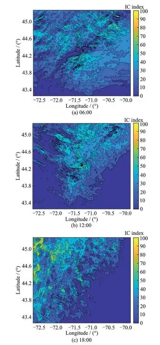
Fig.7 IC index contours of layer η=6 at different time on April 1st in Case 1

According to the definition of the IC index，the icing intensity forecast results can be classified into four categories：No icing，light icing，moderate icing，and severe icing.The specific classification criteria are shown in Table 3.During moderate icing，high rates of accretion on the airframe may cause airspeed loss，which may worsen into severe icing if the aircraft remains exposed to icing for an extended period of time.Therefore，in the case of moderate icing，it is important to activate the aircraft’s anti-icing system or perform evasive maneuvers that may significantly impact the aircraft’s performance［27］.

Fig.8 IC index contours of different altitude layers at 06:00 on April 1st in Case 1

Table 3 Aircraft icing intensity classification

To evaluate different cloud microphysical schemes，the IC index threshold of 50 is selected.This means that a region is at moderate/severe icing risk when the IC index exceeds this threshold.Subsequently，the spatial points within the target region，which is the innermost region of the icing weather prediction，are screened.Fig.9 presents a group of comparisons of the number of spatial grid points that satisfy the moderate icing condition at different height layers at 06：00，12：00，and 18：00 on April 1st.As shown in Fig.9，icing risk areas of varying degrees are present at different time as the altitude layer increasing.The icing risk areas at 06：00，12：00，and 18：00 are mainly concentrated in height layers ofη=5—14 and show a trend of increasing and then decreasing.In general，the predictions by the Milbrandt and Thompson schemes show a more exaggerated performance，compared to those of the Morrison configuration.Conversely，the predictions by the WSM6 scheme are more conservative besides at 18：00.

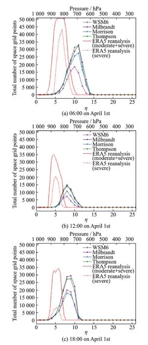
Fig.9 Comparison of total number of space grid points reaching moderate icing intensity at different altitudes in Case 1

Meanwhile，to validate four microphysics schemes，ERA5 reanalysis data with 0.25° horizontal grid spacing resolution provided by the European Centre for Medium-Range Weather Forecasts（ECMWF）is utilized.With the WRF preprocessing system.ERA5 reanalysis data is interpolated into the innermost domain，and the spatial points reaching moderate icing risk are screened.Although this method may overlook subtle variations in the local atmosphere and further overestimates the number of spatial points in the risk zone，it is a reliable way to verify the trends of along the altitude in the icing risk area.In Fig.9，the red solid and dash line indicate the number of interpolated spatial points reaching moderate and severe icing intensity，respectively.All four microphysics schemes overestimate the height level of the icing risk zone.

Further analysis of the IC index contours under four microphysics schemes is shown in Fig.10.Similar to the previously conclusions，the icing intensity predicted by the Milbrandt and Thompson schemes are more serious compared to that by mean of the Morrison scheme，while the results of the WSM6 scheme are milder，particularly in the southern part of the target area.

Fig.10 IC index contours of layer η=11 at 06:00 on April 1st with four microphysics schemes in Case 1

To further investigate the reason for the overestimation，the temperature，relative humidity and IC index at the center point of the target area at 06：00 on April 1st in Case 1 are plotted along the altitude in Fig.11.In Case 1，all four microphysics schemes accurately predict the trend of temperature and relative humidity along the altitude，but the predicted values are generally higher than the ERA5 data.For example，the ERA5 data shows a temperature of-14 ℃ at about 730 hPa isobaric surface，while the predicted temperature of all four schemes decreases to this value only at about 600 hPa isobaric surface.Additionally，the numerical accuracy of relative humidity is also underestimated.It is also shown that the sensitivity of each scheme to RH is different，and the reason for this may lie in the description of different cloud microphysics schemes and the treatment of specific cloud microphysics processes.These above-mentioned discrepancies also lead to the overestimation of the height level of the icing area in some extent.

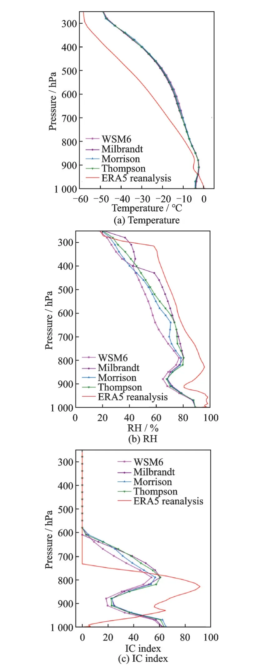
Fig.11 Variation of temperature,RH,and IC index along the altitude at 06:00 on April 1st in Case 1

As shown in Figs.12，13，a similar analysis as in Case 1 is carried out for Case 2.Case 2 is different from Case1 in that rime measurements are interrupted mid-campaign by a rain event，and therefore Case 1 provides an opportunity to assess whether or not the simulations can switch gears from riming conditions to rain and back［22］.Due to the rainfall，the icing risk area in Case 2 is relatively more concentrated near the ground，with a large icing area at 800—700 hPa at 06：00 on March 10th in particular.Although there is still an overestimation of the height of the icing area，the numerical accuracy in Case 2 is very close to the ERA5 data，especially at 06：00 on March 10th and 12：00 on March 12th.

Fig.12 Comparison of total number of space grid points reaching moderate icing intensity at different altitudes in Case 2

In the analysis of temperature，RH，and IC index in the variation along the elevation in Case 2 are shown in Fig.13，and similar conclusions as in Fig.11 can be drawn.Compared to about 690 hPa where the temperature of the ERA5 data reduces to-14 ℃，the predicted temperature by four microphysics schemes decreases to this limitation until 500 hPa isobaric surface，which leads to a wider range of predicted icing risk areas in the altitude direction.Besides，the underestimated but consistent trend of RH predictions also causes deviations between the actual and predicted icing intensity.

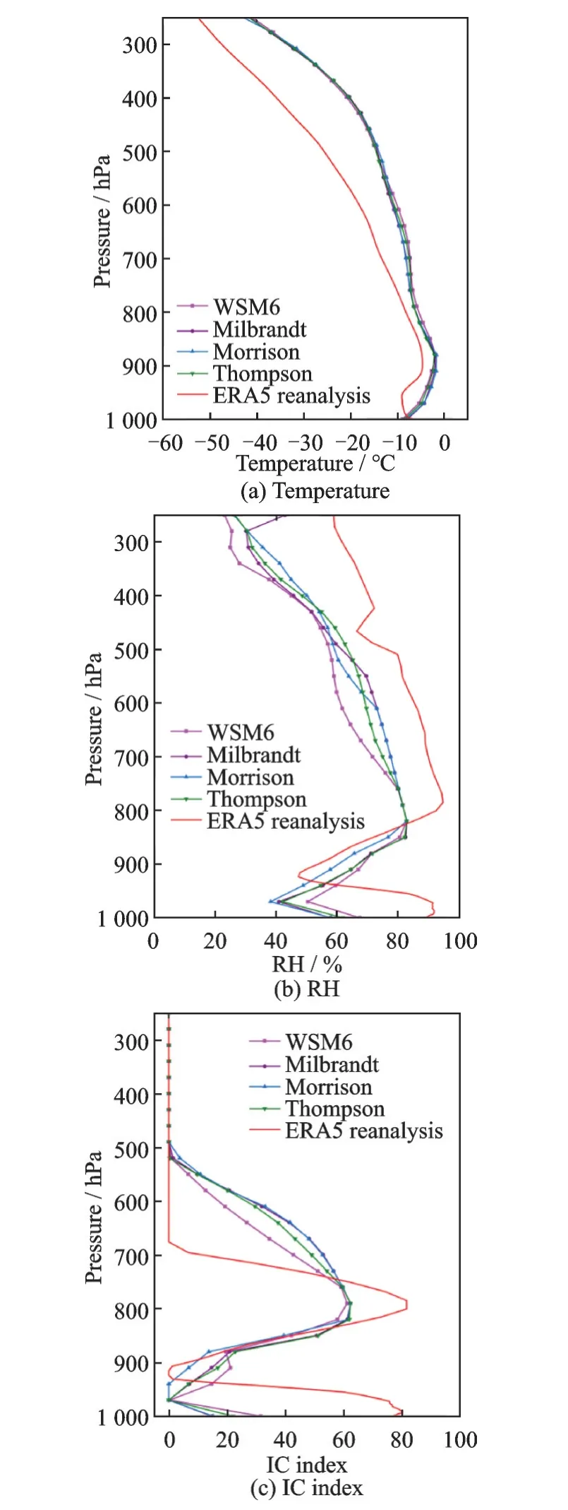
Fig.13 Variation of temperature,RH,and IC index along the altitude at 06:00 on March 10th in Case 2

4 Conclusions

The performance of four cloud microphysics schemes is evaluated based on the simulations of two icing events on Mt.Washington in the U.S.，and the spatiotemporal variability of icing severity under simulations with different microphysics schemes is also assessed utilizing the IC icing index.Some conclusions could be drawn as follow：

（1）LWC and temperature values predicted by the outstanding WRF model are validated and the Morrison configuration obtains the most significant performance in the error analysis.

（2）In addition to the cloud microphysics scheme，horizontal resolution is also a key element for successful prediction，because terrain-induced vertical motions with the finer horizontal resolution are more beneficial for the prediction of cloud water.

（3）The icing severity exhibits a very pronounced spatiotemporal variability and sensitivity to cloud microphysics scheme.The reason for deviations of icing intensity between the prediction and ERA5 reanalysis data is initially interpreted.Meanwhile，in view of the various shortcomings of the IC index algorithm，a more accurate icing intensity forecasting algorithm should be investigated in future.