Unpredictability of Digital Twin for Connected Vehicles
2023-03-12XiaoxuWangZeyinHuangSongmiaoZhengRongYuMiaoPan
Xiaoxu Wang,Zeyin Huang,Songmiao Zheng,Rong Yu,*,Miao Pan
1 School of Automation,Guangdong University of Technology,Guangzhou 510006,China
2 Electrical and Computer Engineering Department,University of Houston,Houston,TX 77004,USA
Abstract: Digital twin is an essential enabling technology for 6G connected vehicles.Through highfidelity mobility simulation,digital twin is expected to make accurate prediction about the vehicle trajectory,and then support intelligent applications such as safety monitoring and self-driving for connected vehicles.However,it is observed that even if a digital twin model is perfectly derived,it might still fail to predict the trajectory due to tiny measurement noise or delay in the initial vehicle locations.This paper aims at investigating the sources of unpredictability of digital twin.Take the car-following behaviors in connected vehicles for case study.The theoretical analysis and experimental results indicate that the predictability of digital twin naturally depends on its system complexity.Once a system enters a complex pattern,its longterm states are unpredictable.Furthermore,our study discloses that the complexity is determined,on the one hand,by the intrinsic factors of the target physical system such as the driver’s response sensitivity and delay,and on the other hand,by the crucial parameters of the digital twin system such as the sampling interval and twining latency.
Keywordst: digital twin; connected vehicles; unpredictability;complexity
I.INTRODUCTION
As an advanced digitalization technology,digital twin is able to replay the past,present the current and predict the future activities of target physical entities in a digital form.Through high-fidelity digital simulation,digital twin builds up an interactive mapping between the physical and digital spaces.People are allowed to observe,assess and control the physical world conveniently via dedicated digital interfaces [1].In the research area of 6G connected vehicles,digital twin has been widely studied for path planning,driving control,trajectory prediction,traffic management,and so on[2,3].Along with deep learning and edge computing[4,5],digital twin has become the essential enabling technology for 6G connected vehicles[6,7].
In most existing work of digital twin for connected vehicles,the mobility simulation in digital space is always supposed to be perfect.The movements of the physical vehicles and that of their digital replicas are well synchronized,such that the deviation between them is considered negligible.However,our observation indicates that sometimes the synchronization between the physical entities and their digital replicas is extremely difficult.Even though a digital twin model is perfectly derived by using state-of-the-art deep learning techniques,the long-term activities of the physical entities might still be unpredictable.For example,considering a car-following scenario,when there is tiny measurement noise or delay in the initial vehicle locations,after a long-time simulation,the movements of vehicles in the digital space might be totally different from that in the physical space.A small imperfect input,e.g.,with noise or delay in location measurement,to the digital twin model might dramatically induce large deviation in mobility simulation,and eventually lead to invalid trajectory prediction.
In this paper,we are motivated to investigate the sources of unpredictability of digital twin for connected vehicles.Without loss of generality,we focus on the vehicle trajectory prediction in car-following scenarios.In particular,we take Bierley and Optimal Velocity Model (OVM) as two typical car-following models for connected vehicles.Mathematically,a digital twin is formulated as a dynamical system governed by Ordinary Differential Equations(ODEs).The crucial digital system parameters such as the sampling interval and twining latency,and the intrinsic physical system complexity such as driver’s response sensitivity and delay,are investigated for their effects to the predictability of digital twin.Theoretical analysis including fixed point analysis,perturbation analysis,bifurcation analysis,and extensive simulation experiments are conducted in our study.The main contributions of this paper are three folds:
・ For a connected vehicles system,we discover that even though its digital twin model is perfectly derived,its long-term activity is not always predictable.A tiny noise or delay in vehicle location measurement might dramatically induce huge deviation in vehicle trajectory prediction.
・ Theoretical analysis and simulation experiments are conducted to investigate the sources of unpredictability of digital twin.We find that the predictability of a digital twin system depends on its complexity.Once the system stays in a complex pattern,its long-term states are unpredictable.
・ Our study further discloses that the complexity is determined,on the one hand,by the intrinsic factors of the target physical system,and on the other hand,by the crucial parameters of the digital twin system such as the sampling interval and twining latency.
The remainder of this paper is organized as follows.Section II introduces the related work of the digital twin for connected vehicles.Section III presents the problem statement,where the system architecture for connected vehicles,the digital twin models and the car-following models are described,respectively.In section IV,we theoretically analyze the trajectory predictability problem under different system conditions such as ideal digital twin model,sampling interval,twining latency and physical complexity.Section V verifies the theoretical analysis by simulation experiments.Section VI summarizes our work in this paper and points out the future direction.
II.RELATED WORK
2.1 Digital Twin for Connected Vehicles
In the literature of digital twin for connected vehicles,many efforts are devoted to improving the driver’s behaviors,driving control,trajectory prediction and path planning,etc.Chen et al.[8]studied the digital behavioral twins for driver’s behaviors of connected vehicles.The potential behaviors of adjacent vehicles were predicted to strengthen driving safety.In[9],driver’s behaviors were found particularly important in mixed traffic flows at non-signalized intersections.Their digital twins could provide satisfying cooperative strategies for vehicles.For driving control,the merging of on-ramp vehicles is a common but challenging problem.In[10],Liao et al.aimed at controlling the connected vehicles in a safe and environmentally sustainable mode with acceptable communication delay by using the proposed digital twin approach.Du et al.[11] focused on trajectory prediction of autonomous intelligent fleets.By leveraging digital twin,the realtime locations of surrounding road users were well estimated.In [12],Hui et al.considered different traffic densities and set rewards to encourage vehicles to comply with scheduling rules for path planning.In this paper,we focus on trajectory prediction for connected vehicles in car-following scenarios.Compared to existing work with interest in performance improvement,our study concentrates on the fundamental problem of the predictability of digital twin for connected vehicles.
2.2 Digital Twin System Implementation
From the perspective of system implementation,digital twin could be created by model-driven [13],datadriven[14]and hybrid-driven approaches[15].
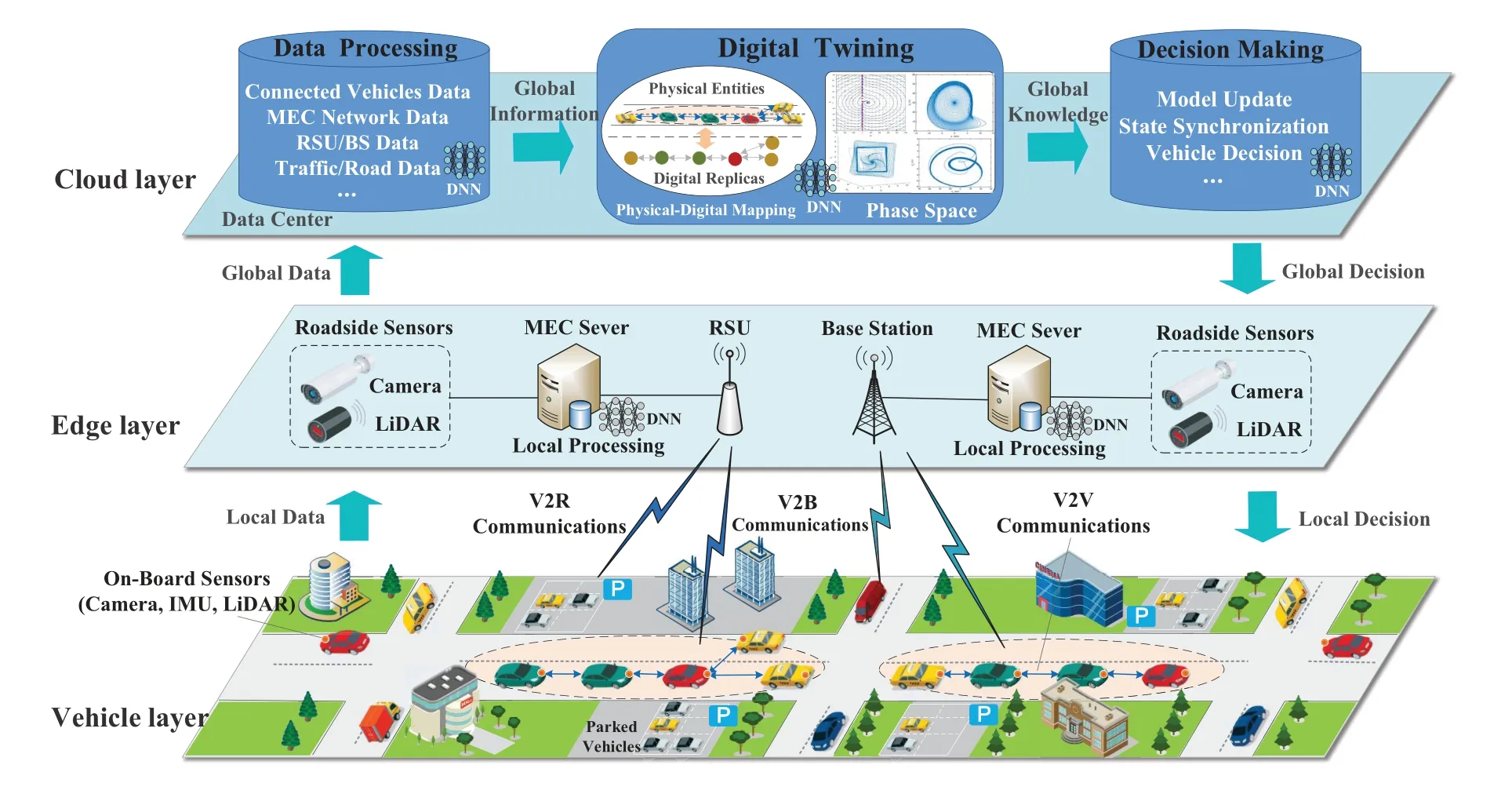
Figure 1.Digital twin system architecture for connected vehicles.
Model-driven digital twin systems are technically derived based on the empirical knowledge about the physical laws and operating rules of the target physical system such as the governing equations.Sun et al.[16]designed digital twins for RSUs and vehicles based on the model of physical entities.Dai et al.[17]proposed a new digital twin network to solve the problem of random computing unloading and resource allocation based on the model-driven.
Data-driven digital twin systems are generated through learning-based approaches using the historical observation data of the target physical system.Lu et al.[18]took the Internet of Things device operation data to construct the digital twin model for communication efficiency enhancement.Sun et al.[19] proposed an architecture of digital twin empowered industrial Internet of things using federated learning.
Hybrid-driven digital twin systems take the advantages of both model- and data-driven approaches to implement high accuracy and efficiency physicaldigital mapping and simulation.The work in[20]integrated the model-driven expert knowledge with datadriven approach,and developed a lightweight digital twin system for smart-cities applications.
As aforementioned,most existing researches tend to improve the accuracy and efficiency of digital twin for a variety of applications.Exploiting model-,dataand hybrid-driven approaches,especially deep learning techniques,for digital twin system implementation is indeed practicably effective.However,it seems that one fundamental problem is ignored.That is,can the predictability of digital twin be theoretically proven?In fact,we observe that even if the system implementation has achieved high accuracy,the model parameter deviation and input data noise can not be completely eliminated.As a consequence,these tiny deviation and noise in digital twin might dramatically lead to considerably large errors in prediction.More concretely,the predictability of digital twin depends not on the implementation approaches,but naturally on the system complexity.In this paper,we attempt to examine the critical conditions that affect the system complexity and deal with the predictability problem of digital twin for connected vehicles.
III.PROBLEM STATEMENT
3.1 System Overview
As shown in Figure 1,we consider a communication architecture for connected vehicles that has a three-tiered network structure of vehicle layer,edge layer and cloud layer.The vehicle layer uses cellular(e.g.,5G and 6G) and V2X (Vehicle-to-Everything)communications to set up the connections of V2V(Vehicle-to-Vehicle),V2R (Vehicle-to-Roadside) and V2B (Vehicle-to-BS,Base Station).The edge layer has MEC(Mobile Edge Computing)servers mounted to the roadside units and base stations.The cloud layer has the data center servers with global information.
Sensors are equipped on vehicles,roadside and intersection infrastructures for physical measurement and scene perception.There are multiple types of sensors such as cameras,IMUs (Inertial Measurement Units),radars,LiDARs(a.k.a.laser radars)and ultrasonic sensors,etc.Sensing data are collected and transmitted to the data center and MEC servers through wireless and wired communications.
The digital twin space is created and maintained jointly by the data center and MEC servers.The data center is in charge of global decision making while the MEC servers are responsible for local decision making.The operation of digital twining has two main steps.The first step is physical-digital mapping,where the physical entities in physical space are projected to the digital replicas in digital space.The second step is phase space simulation that imitates the object movement and trajectory evolution in the phase space.As a consequence,the digital twin is capable of performing high-fidelity mobility simulation for driving safety evaluation,road scene monitoring,traffic event forecast,optimal transportation control,and so on.
3.2 Digital Twin Model
In a digital twin system,the events in a physical space are mapped to that in a digital space.Mathematically,an event in aK-dimensional physical space is denoted as (X,t),where X∈RKis the phase (a.k.a.state),andt ∈R stands for the continuous time.Meanwhile,an event in aK-dimensional digital space is denoted as(X,n),wheren ∈Z stands for thediscrete time.The operation of a target physical system could be depicted by a continuous-time dynamical system with an ordinary differential equation(ODE)as follows:
where Xn=X(n∆t)is the phase at discrete timen,andT: RK →RKis a continuous map derived from Eq.(1).A general form of Eq.(2)is expressed as
3.3 Car-Following Model
Car following is one of the most common transportation phenomena in connected vehicles.It describes the quantitative relations of movements of sequential vehicles [22,23].A variety of car-following models have been proposed and studied,such as General Motor(GM),Bierley model[24,25],Optimal Velocity Model (OVM) [26],Intelligent Driver Model (IDM)and their enhanced models[27,28].In this paper,we will take two fundamental car-following models:Bierley model and the OVM for case study.
3.3.1 Bierley Model
In Bierley model,considering a straight lane,the relations of location,velocity and acceleration of adjacent vehicles are given by[29]
wherexm(t),(t)and(t)denote the location,velocity and acceleration of them-th vehicle (m ∈N)at timet,andα,βandDare the drivers’ response sensitivity coefficient,headway sensitivity coefficient and nominal safety distance between two adjacent vehicles,respectively.Notice thatαandβmay have different values for different vehicles in practice.
3.3.2 Optimal Velocity Model
In OVM,drivers are supposed to maneuver vehicles for reaching expected optimal velocities.The vehicle acceleration in OVM has the following form[30]:
whereτ0andα0are the drivers’ response delay and response sensitivity coefficient,respectively,andV(·)is the velocity optimization function.Letdm=xm −xm+1denote the distance between them-th and(m+1)-th vehicles,the velocity optimization function is empirically given by
where tanh(·)is the hyperbolic tangent function.
IV.THEORETICAL ANALYSIS
In this section,we investigate the predictability of digital twin under different conditions.As a baseline,the system with ideal digital twin model is first analyzed.After that,the effects of non-ideal digitalization conditions such as sampling interval,twining latency,and the intrinsic physical system complexity are examined one after another.
4.1 Predictability of Ideal Digital Twin
An ideal digital twin system will perfectly reflect the target physical system.It is supposed to have sufficiently small sampling interval ∆tand precise parameter fitting off(·)in(3),such that in theoretical analysis,its discrete-time expression could be replaced by the continuous-time one in(1)for convenience.Here,we consider the Bierley car-following model in (4)with three vehicles.Letdm(t)=xm(t)−xm+1(t)andum(t)=(t)−(t) denote the head distance and relative velocity between them-th and(m+1)-th vehicles(m=1,2),respectively.Specifically,We set
The head vehicle is supposed to have a constant velocity(t)=0.The accelerations of the second and the third vehicles are expressed as
Substituting Eq.(8) into Eq.(7),the system is described by the following ODEs:
4.1.1 Fixed Point Analysis
Using the technique of linearization,Eq.(9) is expanded at the fixed point as below:
where X is the vector notation of(d1,u1,d2,u2),and A is the Jacobian matrix given by
The eigenvalue equation of Eq.(10)is expressed as
whereλis the eigenvector notation of(λ1,λ2,λ3,λ4),and I is the identity matrix.By solving(12),we get
Whenα2−4βD2≥0,all eigenvalues are negative real numbers.The fixed point is a stable attractor as shown in Figure 2a.Whenα2−4βD2<0,the four eigenvalues are two pairs of conjugate complex numbers with negative real parts.The phase diagram appears like a stable inward spiral as that in Figure 2b.It is apparent that in all cases the real parts of all eigenvalues are negative.As a consequence,the fixed point is a stable one,which the phase trajectories always converge to.
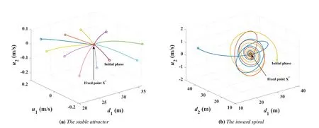
Figure 2.The phase diagram of ideal digital twin for Bierley model.
The fixed point analysis with the phase diagram in Figure 2 presents a sketch about the operating orbits of an ideal digital twin,which roughly reflects the complexity of the system.Strictly speaking,the technique of linearization in(10)works only for the phases close to the fixed point.To examine the trajectories in entire phase space,we conduct perturbation analysis below.
4.1.2 Perturbation Analysis
Consider an initial phase X of the target physical system and a small perturbationϵintroduced by measurement noise or quantization error.The phase of the digital twin is written as=X+ϵ.The ODEs of both X andtake the form of (9).Asϵ=−X,the expression ofϵcould be obtained as
which has four fixed points atϵ∗1=(0,0,0,0),ϵ∗2=andϵ∗4=(−d1,0,0,0),respectively.
Again,we apply linearization to expand Eq.(14)at the fixed points and calculate their eigenvalues to judge the convergence or divergence.For ease of illustration,we represent the original four-dimensional space (d1,u1,d2,u2) jointly by two two-dimensional planes,i.e.,(d1,u1) and (d2,u2),as shown in Figure 3.Each plane is split into three areas,say,A1,A2,A3in (d1,u1) plane,andA′1,A′2,A′3in (d2,u2)plane,whereHere,0< ηt ≪1 and 0< ηt′ ≪1 depend on the perturbationϵ(t).As shown in Table 1,the four-dimensional space is separated into 9 regions withe respect to the initial phase asRk=Ai×A′j,fori ∈{1,2,3},j ∈{1,2,3}andk=3(i −1)+j,where notation×is for the operator of Cartesian product.Accordingly,the fixed point property and phase trajectory evolution are listed.
4.1.3 Discussion on Predictability
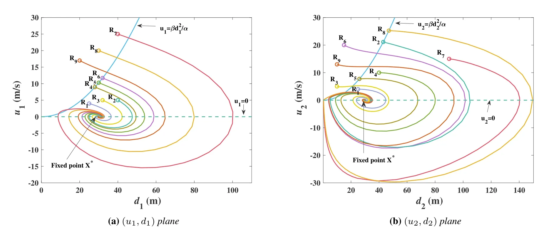
Figure 3.The phase trajectories of different initial phase regions.
The system’s phase trajectory will evolve under the influence of the four fixed pointsϵ∗1,ϵ∗2,ϵ∗3andϵ∗4.Each phase region has one dominant fixed point that decides the convergence or divergence of the perturbation.By tracking the trajectories of different initial phase regions,we know that all of them will eventually go intoR1and converge to the fixed pointϵ∗1,as reported in Table 1.This implies thatϵ →0,and equivalently,→X,as shown in Figure 3.For any initial phase,the trajectory of the target physical system is predictable by that of the digital twin system.From both the fixed point and perturbation analysis,we know that the ideal digital twin of Bierley model is a“simple”system.Its trajectory predictability is theoretically guaranteed.
4.2 Unpredictability Due to Sampling Interval
Now we investigate how the sampling interval affects the predictability of digital twin.As the sampling interval ∆tis not too small to neglect its effect,we have to represent the digital twin as Eq.(3).Also take the Bierley model for case study and consider a fleet with three vehicles.Letdm,n=xm,n −xm+1,ndenote the head distance between them-th and(m+1)-th vehicles andvm,nthe velocity of them-th vehicle at discrete timen(m=1,2).From Eq.(7),we have
wheream,n=+β(dm−1,n−D)denotes the acceleration of them-th vehicle at discrete timen.
Letym,n=Eq.(15)yields
wherer=It is clear that 0<<1 so that 0< ym,n <1.Eq.(16) is the standard form of Logistic map [31].When the system reaches an equilibrium,we havedm,n→∞=D,vm,n→∞=V,and then
whereVis a constant that denotes the vehicles’velocity at equilibrium.It turns out that the increase of ∆twill directly enlarger.
4.2.1 Bifurcation Analysis
In Logistic map,ris a crucial parameter controlling the complexity of the nonlinear system.Changing the value ofrwill lead to the system bifurcation.Foryn+1=ryn(1−yn),the value ofy∞(i.e.,yn→∞)with respect to that ofris described as follows:
・ When 0< r <3,the value ofy∞will always converge to the fixed point.
・ When 3≤r <3.569946,the period doubling occurs.For period 2 (r=3),y∞will oscillate between two specific values.Asrincreases,periods 21,22,23,···,appear one after another.For a given period number,y∞will shift among the corresponding number of values in each cycle.
・ When 3.569946≤r <3.828432,the chaotic phenomenon shows up.The value ofy∞is nearly random in chaos.Meanwhile,along with thechaos,the periodical vibration ofy∞in a finite number of values will be observed sporadically.

Table 1.Perturbation analysis and trajectory evolution.
・ When 3.828432≤r <4,the famousperiod threeemerges atr=3.828432 wherey∞stays in a three-value cycle,and then its period doubling will take place asrincreases.Shortly afterwards,the system will enter chaos again.
・ Whenr ≥4,the system goes into complete chaos.The variation ofy∞is totally disordered.
Note that,due to the sensitivity in parameter accuracy,numbers are rounded to 6 decimal places for the value ofr.The above results tell us thatrth=3.569946 is a critical threshold.Whenr < rth,y∞will converge to the fixed point such that the phases{dm,n,vm,n}could be certainly derived by the digital twin system.But whenr ≥rth,y∞is almost random in chaos.The corresponding phases{dm,n,vm,n}will show up as random value in the digital twin system.
4.2.2 Discussion on Predictability
In digital twin,ris highly dependent on the sampling interval ∆t.Besides the relation in(17),we expect to know more about how ∆taffects the value ofr,and consequently,the predictability of trajectory in digital twin system.Sincervaries with discrete timen,we can rewrite it asrnand define
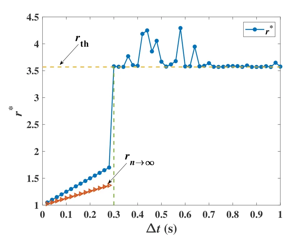
Figure 4.The value of r∗in terms of ∆t with parameter settings: {α1,α2,β1,β2,D,d1,0,d2,0,u1,0,u2,0}={42,33,0.0008,0.0008,12,6,6,0,0}.
Notice thatr∗has selected out the most essential component in{rn} to emphasize the effect ofrth.The value ofr∗in terms of ∆tis shown in Figure 4.We see that when ∆t <0.3,the value ofrnwill never exceed the critical valuerth,i.e.,r∗< rth.For comparison,the value ofr∞(i.e.,rn→∞) is also plotted.Bothr∗andr∞are linear to ∆tfor ∆t<0.3,andr∞is verified to follow(17).When ∆t ≥0.3,some value ofrnwill be larger thanrth,i.e.,r∗≥rth.
All these facts indicate that the digital twin system with a small interval,say,∆t <0.3 in our example,has steady convergence such that its phase trajectory is predictable.On the contrary,the digital twin system with a large sampling interval,say,∆t ≥0.3 in our example,will easily enter chaos,leading to the unpredictability of the phase trajectory.
4.3 Unpredictability Due to Twining Latency
Next we investigate the effect of twining latency on the predictability of digital twin.In a digital twin system as shown in Figure 1,there are communication delay from the onboard and roadside sensors to the edge and cloud servers,and computation duration for model derivation and simulation.We refer to the total time cost of in communication and computation for digital twin operation and maintenance astwining latency.Typically,it is generated when using online reinforcement learning or federated learning among the center and edge servers to estimate and update the model parameters.The Bierley model with twining latencyτis given by
4.3.1 Fixed Point Analysis
The unique fixed point of Eq.(20) is (D,0,D,0).By applying linearization technique at the fixed point,Eq.(20)can be expressed as
where X(t)=(d1(t),u1(t),d2(t),u2(t)).Matrix A and B are given by
Letp(λ,τ)=det(λI−A−Be−λτ)denote the eigenvalue equation.By settingp(λ,τ)=0,we have
For Eq.(22),whenτ=0,all eigenvalues are negative real numbers.The system is stably converged.This fact coincides with the result in Section 4.1 that,for Bierley car-following behavior,an ideal digital twin model (e.g.,with sufficiently high sampling interval and zero twining latency) has low complexity and converged phase trajectory.But ifτ >0,the operation of the system’s phase trajectory has complex pattern,for which we conduct the following bifurcation analysis.
4.3.2 Bifurcation Analysis
For problem (20) and its eigenvalue equation (22),whenτincreases from zero,the system may have complex eigenvalues that will go through the imaginary axis and enter the right half complex plane.In this case,bifurcation will occur.Mathematically,the condition for bifurcation is expressed as
whereistands for the unit of imaginary number.By Eqs.(22)and(23),we have
Squaring both the left-hand sides of Eqs.(24a) and(24b)and adding them up,yield
which has a unique positive real solution
Substitute Eq.(26)into Eq.(24b)to get a general expressionτ∗=k ∈Z+,where arctan(·) is the inverse tangent function.Since we are interested in the minimal critical twining latency,letk=0 and then have
To examine the effect ofτto the change of eigenvalueλ,we calculate the derivative ofλoverτand take its real part atτ=τ∗as follows
which has a positive definite value.This verifies that,with the change ofτ,the eigenvalues of(22)will cross the imaginary axis at a non-zero velocity.This is a sufficient condition for the occurrence of Hopf bifurcation[32].Since Hopf bifurcation is a key route for a system to enter a complex pattern,we can say that the twining latencyτ∗in (27) is a critical value for triggering the complexity in the digital twin system.
4.3.3 Discussion on Predictability
From the fixed point analysis and bifurcation analysis,we know that when 0≤τ < τ∗,the fixed point(D,0,D,0) is a stable one.The system has a converged phase trajectory.Whenτapproachesτ∗,the fixed point is surrounded by a four-dimensional saddle ring with two-dimensional stable and two-dimensional unstable flows.Whenτ=τ∗,the system has four eigenvalues with two negative real ones and two pure imaginary ones.There is an unstable limit cycle with the occurrence of Hopf bifurcation.Meanwhile,the fixed point becomes a saddle point,and the original stable attractor become unstable.Whenτ > τ∗,all eigenvalues of the system have positive real parts.The unstable attractor become a strange attractor.The system no longer has steady convergence and enters the chaotic region,showing a complex pattern.
In summary,for 0≤τ < τ∗,the system’s phase trajectory is converged and predictable.The trajectory in the digital space is well synchronized to that in the physical space.But forτ ≥τ∗,the system’s phase trajectory is not converged,such that the trajectory in the digital space twin fails to present a valid prediction for that in the physical space.
4.4 Unpredictability Due to Physical System Complexity
From Section 4.1,we know that an ideal digital twin for a “simple” target physical system,e.g.,Bierley model,has fine predictability.In this Section,we will show that an ideal digital twin for a“complex”target physical system may lose its predictability.Specifically,take the OVM car-following model for example.Eq.(5)has shown that,the driver’s response delayτ0and response sensitivity coefficientα0are two intrinsic parameters tightly related to the physical system complexity.Our discussion will focus on the relation ofα0andτ0to the predictability of digital twin.
Consider an OVM car-following scenario of a fleet with three vehicles.Letdm(t)=xm(t)−xm+1(t)andum(t)=(t)−(t) denote the head distance and relative velocity between them-th and (m+1)-th vehicles(m=1,2),respectively,and(t)=v0,(t)=0.The target physical system is governed by Eq.(5).Its ideal digital twin system could be expressed as the ODEs below:
4.4.1 Fixed Point Analysis
Eq.(29)has a unique fixed point(d∗,0,d∗,0),where
and artanh(·)the inverse hyperbolic tangent function.LetV ′=|dm=d∗=1.4448−1.4448(−0.913)2,form={1,2}.Using linearization technique and expanding Eq.(29)at the fixed point yield
where X(t)=(d1(t),u(t),d2(t),u2(t)).The matrix A and B are given by
Letp(λ,α0,τ0) denote the eigenvalue equation of Eq.(31),i.e.,p(λ,α0,τ0)=det(λI−A−Be−λτ0).Settingp(λ,α0,τ0)=0,we get
From Eq.(6),we know thatV ′ >0.For Eq.(32),ifα0=0 orτ0=0,all the eigenvalues are negative real numbers,and therefore,the system is stably converged,as Routh-Hurwitz criterion tells [33].However,neitherα0=0 norτ0=0 is realistic.We have to consider the case ofα0>0 andτ0>0.In fact,the increase ofα0andτ0will trigger the system bifurcation as discussed below.
4.4.2 Bifurcation Analysis
As the values ofα0andτ0change,the eigenvalues of Eq.(32)might cross over the imaginary axis and go to the right half of the complex plane,inducing the system bifurcation.Mathematically,the bifurcation condition is expressed as
whereiis the unit of imaginary number.Substitutingλ=±iω0to Eq.(32)yields
Combining Eqs.(34a)and(34b),we obtain
When given a value ofα0,by solving Eq.(35),we have the critical value ofω0as
and the critical values ofτ0asτ∗0=k ∈Z+.Letk=0 to keep the minimal critical value
In Eq.(32),we calculate the derivative ofλoverτ0,and obtain its real part atτ0=τ∗0as below:
Apparently,Eq.(38)is positive definite,which means that,with the increase ofτ0,the eigenvalues of (32)will go through the imaginary axis at a non-zero velocity,satisfying the transversal condition of Hopf bifurcation.
Substituting Eq.(36) into Eq.(37),we derive the critical relation ofτ∗0andα∗0for Hopf bifurcation as
In other words,for a given pair of (α0,τ0),we know that the target physical system is a complex one if
4.4.3 Discussion on Predictability
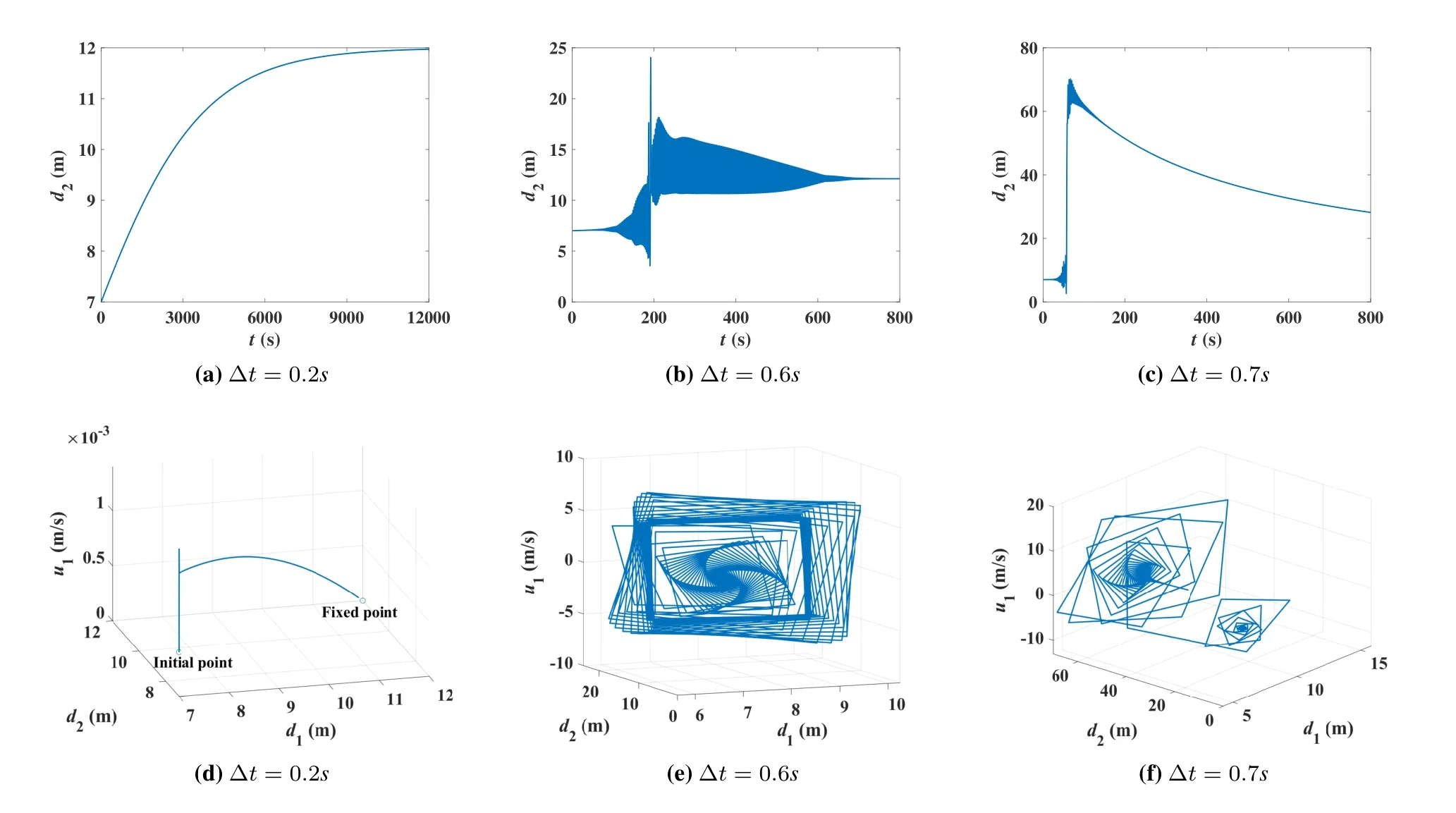
Figure 5.Effect of sampling interval to the trajectory evolution in digital twin.
As mentioned before,in the OVM car-following scenario,the driver’s response sensitivity and delay,α0andτ0,are two intrinsic parameters determining the physical system complexity.Provided a pair of(α0,τ0),if they are small so that Eq.(40) doesn’t hold,the fixed point (d∗,0,d∗,0) is a stable one,to which the phase trajectory will converge.The ideal digital twin system is able to present a fine prediction of the phase trajectory.But if (α0,τ0) is closely approaching (α∗0,τ∗0) that satisfies Eq.(39),the fixed point in the phase space is surrounded by a four dimensional saddle ring with two-dimensional stable and two-dimensional unstable flows.If (α0,τ0) exactly reaches(α∗0,τ∗0),there is an unstable limit cycle.Hopf bifurcation occurs and the original attractor becomes unstable.If (α0,τ0) is large so that the inequality in(40)strictly holds,the strange attractor emerges.The physical system will enter a chaotic pattern[32].Even the ideal digital twin could not present valid prediction on the phase trajectory of the target physical system.
V.EXPERIMENTAL EVALUATION
In this section,we evaluate the predictability of digital twin for car-following scenarios under different conditions,including sampling interval,twining latency and physical system complexity,respectively.
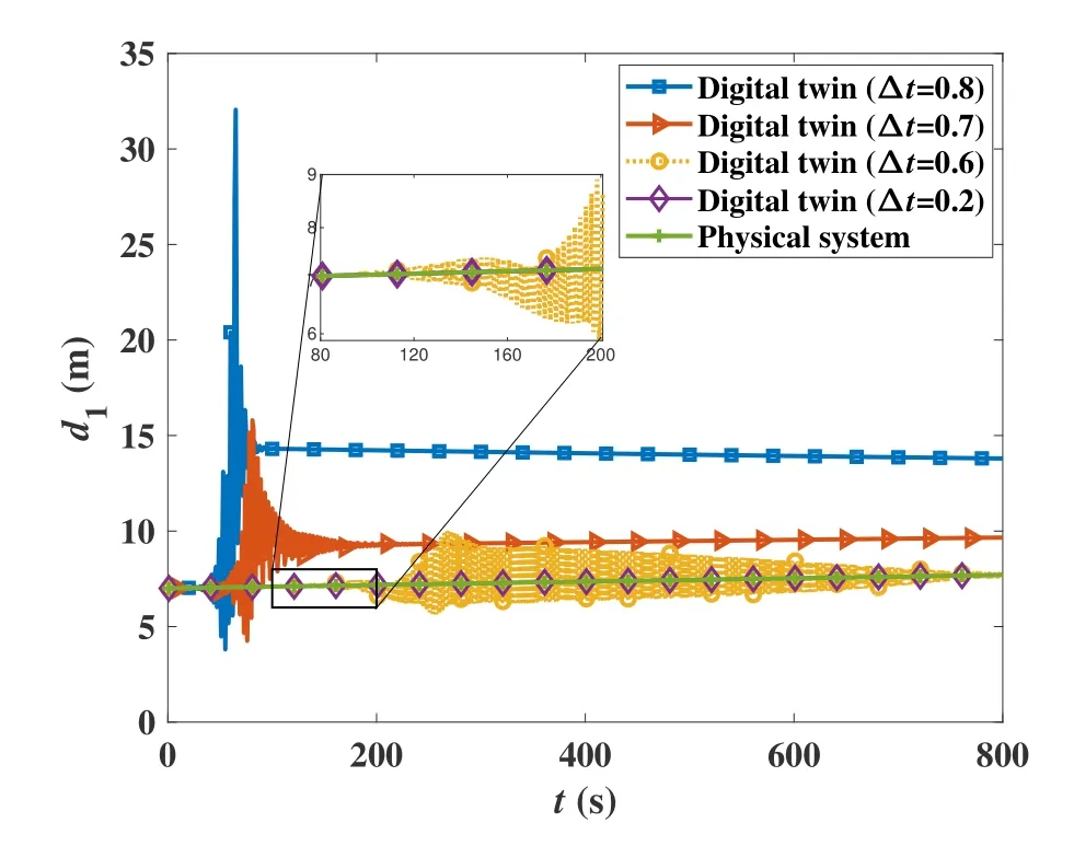
Figure 6.Comparison of predictability of digital twin under different sampling intervals.
5.1 Effect of Sampling Interval
In this experiment,we consider the Bierley carfollowing scenario of a fleet with three vehicles as that in Eq.(15).Let nominal safety distanceD=12m,response and headway sensitivity (α,β),i.e.,(25,0.0008) and (20,0.0008) for the middle and last drivers,respectively.The initial headway and velocity are set tod1,0=d2,0=7m andv1,0=v2,0=15m/s.Three groups of tests with sampling intervals ∆t=0.2s,0.6s and 0.7s,respectively,are conducted to examine the effect of sampling interval to the trajectory evolution.The result is reported in Figure 5.In addition,a group of tests are carried out to compare the predictability under sampling intervals 0.2s,0.6s,0.7s and 0.8s,as shown in Figure 6.
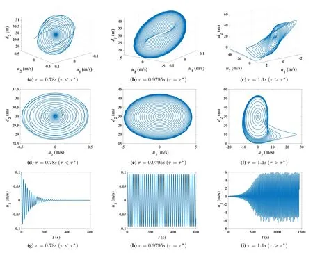
Figure 7.Effect of twining latency to the trajectory evolution in digital twin.
In Figure 5,the curves of headwayd2in terms of timetare plotted in Figures 5a,5b and 5c for sampling intervals ∆t=0.2s,0.6s and 0.7s,respectively.The trajectories in the three-dimensional phase space(d1,d2,u1) are shown in Figures 5d,5e and 5f for∆t=0.2s,0.6s and 0.7s,respectively.It is observed that,for ∆t=0.2s,the headwayd2will gradually converge to the equilibrium value at the fixed point,say,d2=D=12m in Figure 5a.The trajectory in the phase space(d1,d2,u1)vibrates shortly at the beginning and then slides smoothly to the fixed point as shown in Figure 5d.For ∆t=0.6s,the headwayd2in Figure 5b has a heavy oscillation,while the trajectory of (d1,d2,u1) in Figure 5e appears as a nested spiral.Clearly,the system has experienced a complex chaotic pattern.For ∆t=0.7s,the sharp oscillation of the curve in Figure 5c and the two vortex-like variation of the trajectory in Figure 5f imply the appearance of strange attractor,which is a key feature of chaos.We know from these results in Figure 5 that once the sampling interval ∆tis large enough,the trajectory of the digital twin system will become chaotic and totally disordered.
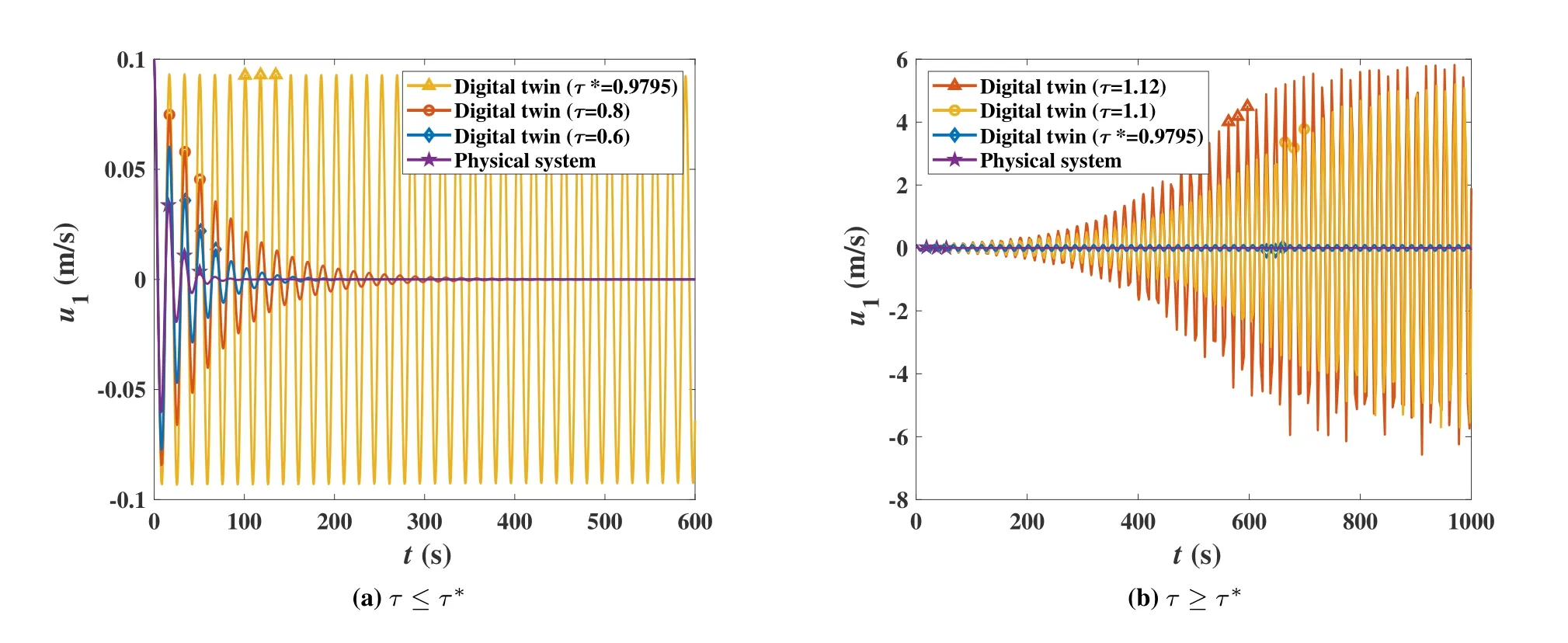
Figure 8.Comparison of predictability of digital twin under different twining latency.
In Figure 6,the predictability of the headwayd2under different sampling intervals ∆t=0.2s 0.6s,0.7s,0.8s are compared.For a small sampling interval∆t=0.2s,the digital twin is able to output accurate values as the groundtruth from the physical system.But for large sampling intervals ∆t=0.6s,0.7s and 0.8s,the output of the digital twin drastically vibrates and severely deviates from the groundtruth.We also find that,among ∆t=0.6s,0.7s and 0.8s,the larger the sampling interval is,the earlier and stronger the vibration comes.Only the small sampling interval,say,∆t=0.2s,could offer fine predictability.
5.2 Effect of Twining Latency
In this experiment,we also consider the Bierley carfollowing scenario of a fleet with three vehicles as that in Eq.(20).Letα=4,β=0.13,D=30m,d1(0)=d2(0)=30m,u1(0)=u2(0)=0.1m/s,andv0=15m/s.As Eq.(27),the critical value for bifurcationτ∗=0.9795s.We examine the trajectory evolution in digital twin under different twining latencyτ=0.78s,0.9795s and 1.1s.The result is presented in Figure 7.Meanwhile,we compare the predictability of digital twin under different twining latencyτ=0.6s,0.8s,0.9795s,1.1s and 1.12s,as reported in Figure 8.
In Figure 7,the trajectory in phase space(d2,u1,u2)and that in phase plane (d2,u2) under latencyτ=0.78s,0.9795s and 1.1s are displayed in Figures 7a,7b,7c,and Figures 7d,7e,7f,respectively.The relative velocityu1in terms of time under latencyτ=0.78s,0.9795s and 1.1s are plotted in Figures 7g,7h and 7i,respectively.We can see that,forτ=0.78s< τ∗,the trajectory spins round and stably converges to the fixed point.The relative velocityu1will oscillate and gradually converge to zero.Forτ=0.9795s=τ∗,the limit cycle appears in this critical case,as shown in Figures 7b and 7e.The curve ofu1has an undamped oscillation as that in Figure 7h.Forτ=1.1s> τ∗,there exists a strange attractor such that the trajectory will diverge at first and then turn to a quasi-periodic oscillation,as Figures 7c and 7f show.The envelope ofu1keeps increasing during oscillation and then remains at an asymptotically equal level as that in Figure 7i.
In Figure 8,we compare the predictability of the relative velocityu1under different twining latency.We select a group ofτ ≤τ∗,say,τ=0.6s,0.8s and 0.9795s in Figure 8a,and a group ofτ ≥τ∗,say,τ=0.9795s,1.1s and 1.12s in Figure 8b.The curves of physical system andτ=τ∗are baselines for comparison in the two figures.It is observed that,for digital twin withτ < τ∗,the value ofu1always converges to the groundtruth of the physical system,before which it has to experience a period of oscillation.In this case,we also see that the larger the twining latency is,the stronger and longer the oscillation takes.Forτ=τ∗0,the curve ofu1has undamped oscillation.Its value fails to predict that of the physical system.Forτ > τ∗0,the curve ofu1oscillates with a growing amplitude before reaching the level with a roughly but not exactly equal range,due to the effect of a strange attractor.The emergence of strange attractor is a sign of chaos,which implies the unpredictability of trajectory.
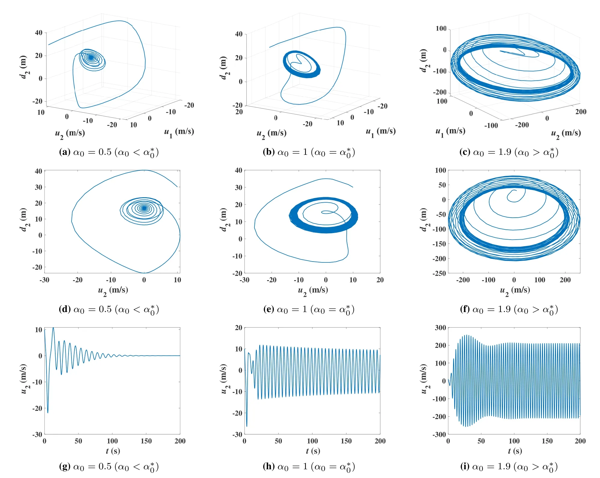
Figure 9.Effect of driver’s response sensitivity to the trajectory evolution in digital twin.
5.3 Effect of Physical System Complexity
This experiment takes the OVM car-following scenario for study.The physical system complexity is determined by the driver’s response sensitivity and delayα0andτ0.The ideal digital twin is formulated by (29).In the scenario of a fleet with three vehicles,letv0=5m/s,d1(0)=d2(0)=30m,u1(0)=u2(0)=10m/s.We examine the effects ofα0andτ0to the trajectory evolution in digital twin in Figures 9 and 10,respectively.Then,we compare the predictability of digital twin under different physical complexity due toα0andτ0in Figures 11 and 12,respectively.
In Figure 9,consider (α∗0,τ∗0)=(1,0.7627) that satisfies Eq.(39).Fix the value ofτ0=τ∗0.The experimental results forα0=0.5,1 and 1.9 are shown in Figures 9a,9d,9g,Figures 9b,9e,9h,and Figures 9c,9f,9i,respectively.In Figure 10,consider(α∗0,τ∗0)=(0.8,0.8217) that follows Eq.(39).Fix the value ofα0=α∗0.The experimental results forτ0=0.6217,0.8217 and 1.0217 are shown in Figures 10a,10d,10g,Figures 10b,10e,10h,and Figures 10c,10f,10i,respectively.We can see that,forα0< α∗0in in Figures 9a,9d,9g,andτ0< τ∗0in Figures 10a,10d,10g,the trajectory forms an inward spiral and converges to the fixed point in phase space(d2,u1,u2)and phase plane(d2,u2).The curve ofu2also vibrates down to zero certainly.Forα0=α∗0in Figures 9b,9e,9h,andτ0=τ∗0in Figures 10b,10e,10h,the trajectory is attracted to walk around the limit cycle in phase space(d2,u1,u2)and phase plane(d2,u2),whileu2wanders shortly and adjusts to an undamped oscillation.Forα0> α∗0andτ0=τ∗0,under the effect of strange attractor,the trajectory is spinning around a randomly perturbed cycle,whileu2is oscillating with an unstable amplitude,as shown in Figures 9c,9f and 9i.Forτ0> τ∗0andα0=α∗0,the strange attractor makes the trajectory jump alternatively between two perturbed cycles,andu2oscillate roughly with two amplitudes,as shown in Figures 10c,10f and 10i.
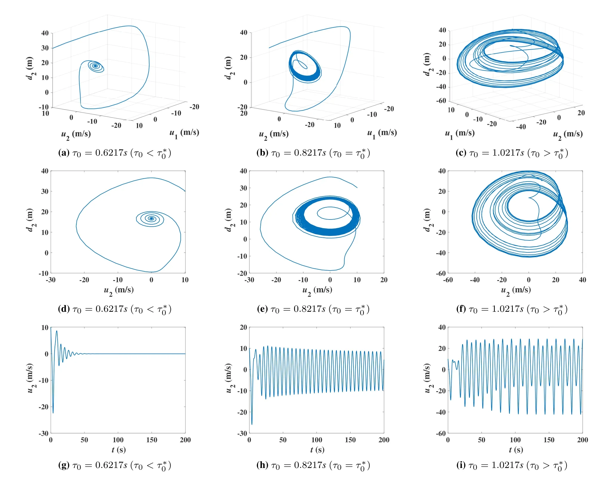
Figure 10.Effect of driver’s response delay to the trajectory evolution in digital twin.
In Figure 11,considering (α∗0,τ∗0)=(1,0.7627),the curves ofu2of digital twin and physical system underα0=0.5 and 1.8 are plotted in Figures 11a and 11b,respectively.Suppose that there is a small deviation in the value ofα0,say,δ=±0.1 due to the bias of parameter fitting in digital twin system.We can see that,forα0=0.5< α∗0,the digital twin can still offer fine prediction of the value ofu2.But forα0=1.8> α∗0,the digital twin fails to offer valid prediction.In Figure 12,considering(α∗0,τ∗0)=(0.8,0.8217),the curves ofu2of digital twin and physical system underτ0=0.62s and 1.21s are plotted in Figures 12a and 12b,respectively.Set a small deviation inτ0asδ=±0.1s due to the parameter bias in digital twin system.We find that,forτ0=0.62s< τ∗0,the digital twin can accurately predict the value ofu2.But forτ0=1.21s> τ∗0,the digital twin is unable to predict the curve ofu2for the physical system.
5.4 Effect of Initial State Deviation
In this section,we investigate the effect of initial state deviation to the predictability of digital twin systems.We rerun the experiments in Sections 5.1,5.2 and 5.3 separately.In each experiment,we compare the trajectories under two different initial states.Specifically,in the three experiments,the state deviationδis added to different variablesdm,0+δ,(m=1,2),u1(0)+δandu2(0)+δ,respectively.Let ∆um,(m=1,2)denote the difference of the relative velocity in the digital twin and that in the physical system.The results for the three experiments are shown in Figures 13a,13b and 13c,respectively.We can observe from all the three figures that,an initial tiny deviation will eventually lead to a considerably large error in trajectory prediction.Furthermore,it seems that the amplitude of the prediction error dose not depend on that of the initial deviation.It is obvious that the system has enter a complex pattern,in which the digital twin fails to predict the behavior of the physical system.
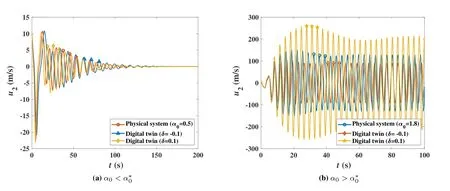
Figure 11.Comparison of predictability of digital twin under different driver’s response sensitivity.
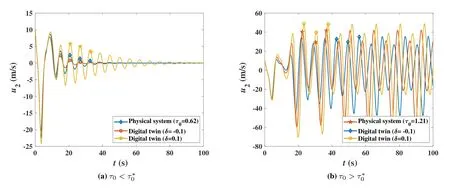
Figure 12.Comparison of predictability of digital twin under different driver’s response delay.
VI.CONCLUSION
In this paper,our study focuses on the sources of unpredictability of digital twin for connected vehicles.Take the vehicle trajectory prediction problem in carfollowing scenarios for case study.Our findings indicate that,the crucial parameters of digital twin system such as sampling interval and twining latency,and the intrinsic factors of target physical system such as the driver’s response sensitivity and delay may inherently induce system complexity and consequently lead to trajectory unpredictability.If the system reaches the critical conditions and enters a complex pattern,the trajectory in the digital space fails to predict that in the physical space,even if a tiny deviation in the initial state or parameter fitting introduced by measurement noise or delay.Theoretical deduction with fixed point analysis,perturbation analysis and bifurcation analysis,and experimental evaluation are conducted to demonstrate the results.Our future work will further investigate the conditions and mechanisms of unpredictability of digital twin,and meanwhile,explore the principles and methods to recover the predictability.
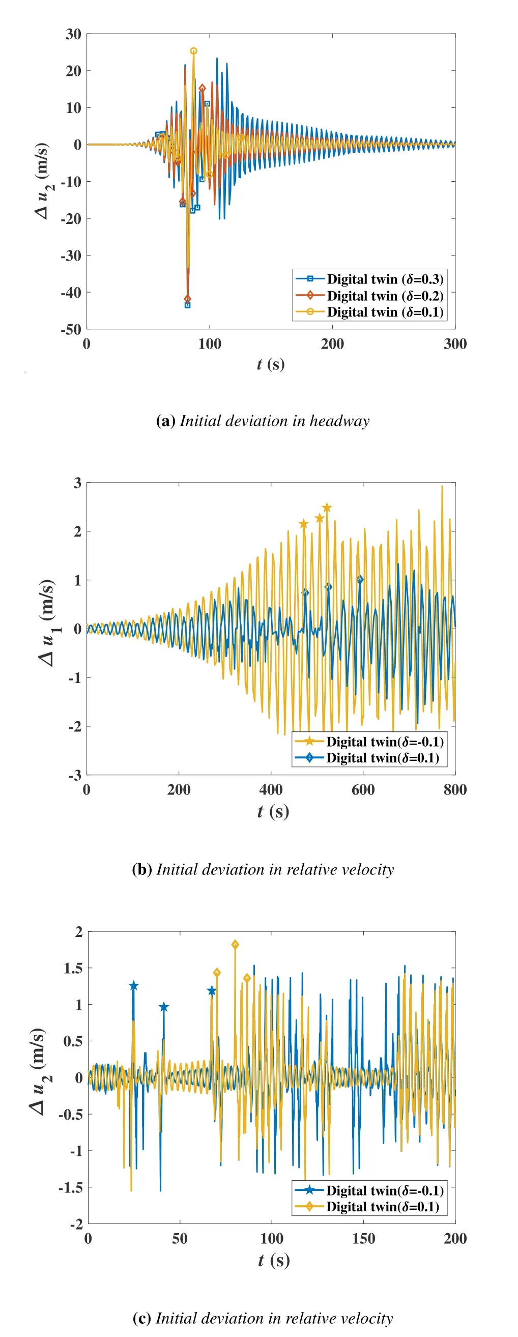
Figure 13.Prediction Errors of digital twin in different initial state deviation
ACKNOWLEDGEMENT
The work is supported in part by National Key R&D Program of China(No.2020YFB1807802),National Natural Science Foundation of China(Nos.61971148,U22A2054).
杂志排行
China Communications的其它文章
- Convergence of Digital Twin and 6G enabled Edge Intelligence: Theories,Algorithms and Applications
- Design and Implementation of Secure and Reliable Information Interaction Architecture for Digital Twins
- The Development Trends and Research Fronts in Orbital Angular Momentum Technology: A Bibliometric Analysis
- A Dynamic Bayesian-Based Comprehensive Trust Evaluation Model for Dispersed Computing Environment
- Research on Network Cognition Model and Mechanism of Intelligent Information Network
- Low-Density Parity-Check Codes: Highway to Channel Capacity
