Damage Curves Derived from Hurricane Ike in the West of Galveston Bay Based on Insurance Claims and Hydrodynamic Simulations

Chaoran Xu · Benjamin T.Nelson-Mercer · Jeremy D.Bricker,4 · Meri Davlasheridze · Ashley D.Ross ·Jianjun Jia

Abstract Hurricane Ike, which struck the United States in September 2008, was the ninth most expensive hurricane in terms of damages.It caused nearly USD 30 billion in damage after making landfall on the Bolivar Peninsula, Texas.We used the Delft3d-FM/SWAN hydrodynamic and spectral wave model to simulate the storm surge inundation around Galveston Bay during Hurricane Ike.Damage curves were established through the relationship between eight hydrodynamic parameters (water depth, f low velocity, unit discharge, f low momentum f lux, signif icant wave height, wave energy f lux, total water depth (f low depth plus wave height), and total (f low plus wave) force) simulated by the model and National Flood Insurance Program(NFIP) insurance damage data.The NFIP insurance database contains a large amount of building damage data, building stories, and elevation, as well as other information from the Ike event.We found that the damage curves are sensitive to the model grid resolution, building elevation, and the number of stories.We also found that the resulting damage functions are steeper than those developed for residential structures in many other locations.

Keywords Delft3d-FM · Flood risk · Hurricane Ike · Residential damage ratio · SWAN · Weibull function

1 Introduction

Hurricanes are highly destructive marine weather systems that are accompanied by gale-force winds, heavy rainfall,and storm surges (Muis et al.2016).This can result in low-latitude coastal zones at lower elevations being highly susceptible to f looding (Tyler et al.2021).It is estimated that 10% of the world’s population lives in the 2% of the total landmass of the Earth that comprises the low-elevation coastal zone, which is vulnerable to storm surge and inundation (Oliver-Smith 2009).In the United States, hurricanes have been responsible for eight of the top 10 costliest disasters since the 1980s (NOAA 2023); globally, the annual hurricane damage is about USD 26 billion (Mendelsohn et al.2012).Meanwhile, because of global warming, more warm and wet seawater evaporates to increase the moisture in the air, which leads to an increase in the intensity of hurricanes and slowing of onshore storm weakening, so coastal areas may suf fer more economic losses in the future (Knutson et al.2019; Li and Chakraborty 2020; Xu, Yang, et al.2022).Storm surge is a major driver of food risk, and coastal development also magnif ies risk by increasing exposure to these hazards (Davlasheridze et al.2019; Reed et al.2020;Davlasheridze et al.2021; Törnqvist et al.2021).The East Coast and Gulf Coast of the United States are regions heavily af fected by storm surges, aggravated by global warming;on these f lat f loodplains, the risk of storm surges can extend several miles inland from the coast, depending on topography, hurricane intensity, and tidal levels during the hurricane(Al-Attabi et al.2023).

Coastal planners need methods to reduce the damage to residences during hurricanes, and the critical f irst step is predicting the relationship between damage and environmental and structural variables.Common environmental forcings associated with hurricane damage include water depth and f low velocity (Tomiczek et al.2017).The damage curve of a building is inf luenced by its structural features, such as the building material, construction methods, codes, and layout, including the distance between buildings (Suppasri et al.2013; Huizinga et al.2017; Masoomi et al.2019;Postacchini et al.2019; Jansen et al.2020).Damage curves are often used to parameterize this relationship and are an important tool for risk assessment related to environmental and structural vulnerability (Pistrika and Jonkman 2009;Englhardt et al.2019).Damage curves have been widely applied in the United States, Europe, and Japan (Suppasri et al.2013; Tomiczek et al.2017; Hatzikyriakou and Lin 2018; Diaz-Loaiza et al.2022).Suppasri et al.( 2013) established damage curves for Japanese coastal zones based on f lood depths for residential structures (including the number of residential f loors and the type of residential construction materials).Tomiczek et al.( 2017) studied the relationship between structural damage state and f low velocity in New Jersey as a result of Hurricane Sandy.However, these studies focused only on a single variable.The National Flood Insurance Program (NFIP) provides a large amount of measured insurance claims data including water depth, the amount of residential damage, the number of residential f loors, and other residential information (FEMA 2023).In the United States, widely used curves have been compiled by the Army Corps of Engineers (USACE) based on NFIP data.However,there are anomalies in the NFIP water depth data, so damage curves based on these lack reliability (Wing et al.2020).

The rapid evolution of f lood hazard modeling techniques,fueled by advances in computer power and the development of high-resolution terrain data, has brought about a transformative shift in our understanding of f lood hazard, even at continental and global scales (Sampson et al.2015; Winsemius et al.2015).While water depth is an important variable as it ref lects the static forces exerted on a structure, in hurricane events, structures located near the coast may also be subjected to dynamic forces, such as the impact of f low and waves (Kreibich et al.2009; Tomiczek et al.2017).Therefore, f lood damage is not only related to the water depth and f low velocity, but six other hydrodynamic parameters (unit discharge, f low momentum f lux, signif icant wave height,total water depth, wave energy f lux, and total force) are also very signif icant (Tsubaki et al.2016; Bricker et al.2017;Diaz-Loaiza et al.2022).However, few studies have been done in this area to provide more perspective on f lood risks in coastal zones (Kreibich et al.2009; De Risi et al.2017;Jansen et al.2020).Hurricane Ike (2008) caused about USD 30 billion in damage, of which insured losses amounted to USD 12.5 billion, and casualties around Galveston Bay,where strong onshore winds and low atmospheric pressure generated unprecedented inundation (Veeramony et al.2016).Therefore, the establishment of damage curves with eight hydrodynamic parameters in this region is important for future disaster mitigation.In this study, we applied the Delft3d-FM numerical model to obtain more accurate hydrodynamic parameters, and through the NFIP database had access to over 20,000 residential claims associated with Hurricane Ike.Therefore, the main objective of the present study was to develop damage curves from NFIP insurance claims data supported by hydrodynamic modeling during Hurricane Ike.

2 Methods

This section begins with an overview of the study area and hurricane Ike.It then covers data sources, introduces the Delft3D-FM, discusses model validation, and outlines the method for damage curve generation.

2.1 Study Area and Hurricane Ike

Galveston Bay is a densely populated, hurricane-prone region.The bay is 50 km long and 27 km wide and is the largest estuary along the Gulf Coast of Texas with a surface area of 1554 km 2.Galveston Bay is shallow, with an average water depth of 3 m, but has a shipping channel of 12 m depth.The San Jacinto and Trinity Rivers are the main sources of fresh water into the bay.On the ocean side,two entrances connect the bay with the Gulf of Mexico (Al-Attabi et al.2023).Hurricane Ike made landfall between Galveston Island and the Bolivar Peninsula (Fig.1) on 10 September 2008, with sustained wind speeds of 130–148 km/h and a surge of 5 m on the Bolivar Peninsula; sustained wind speeds of 120–130 km/h and a surge of 3.5 m on Galveston Island (Overpeck 2009; Sebastian et al.2014).Although it had weakened to a Category 2 storm when it made landfall, its strong wind f ield caused a large storm surge in Galveston Bay, causing severe f looding hazards and major destruction of coastal properties.Hurricane Ike directly caused about USD 30 billion in damage and 12 fatalities in this region (Berg 2009).Since most of the population is concentrated on the western shore of the bay and the east is mostly coastal wetlands, the economic loss on the west shore is greater than that on the east shore (Al-Attabi et al.2023).Therefore, this study focused on the western region of Galveston Bay and established damage curves for the western shore of the bay (Fig.1).

2.2 Hydrodynamic Model of Hurricane Ike

This section introduces the data sources, Delft3D-FM model, and its settings, and presents validation results.

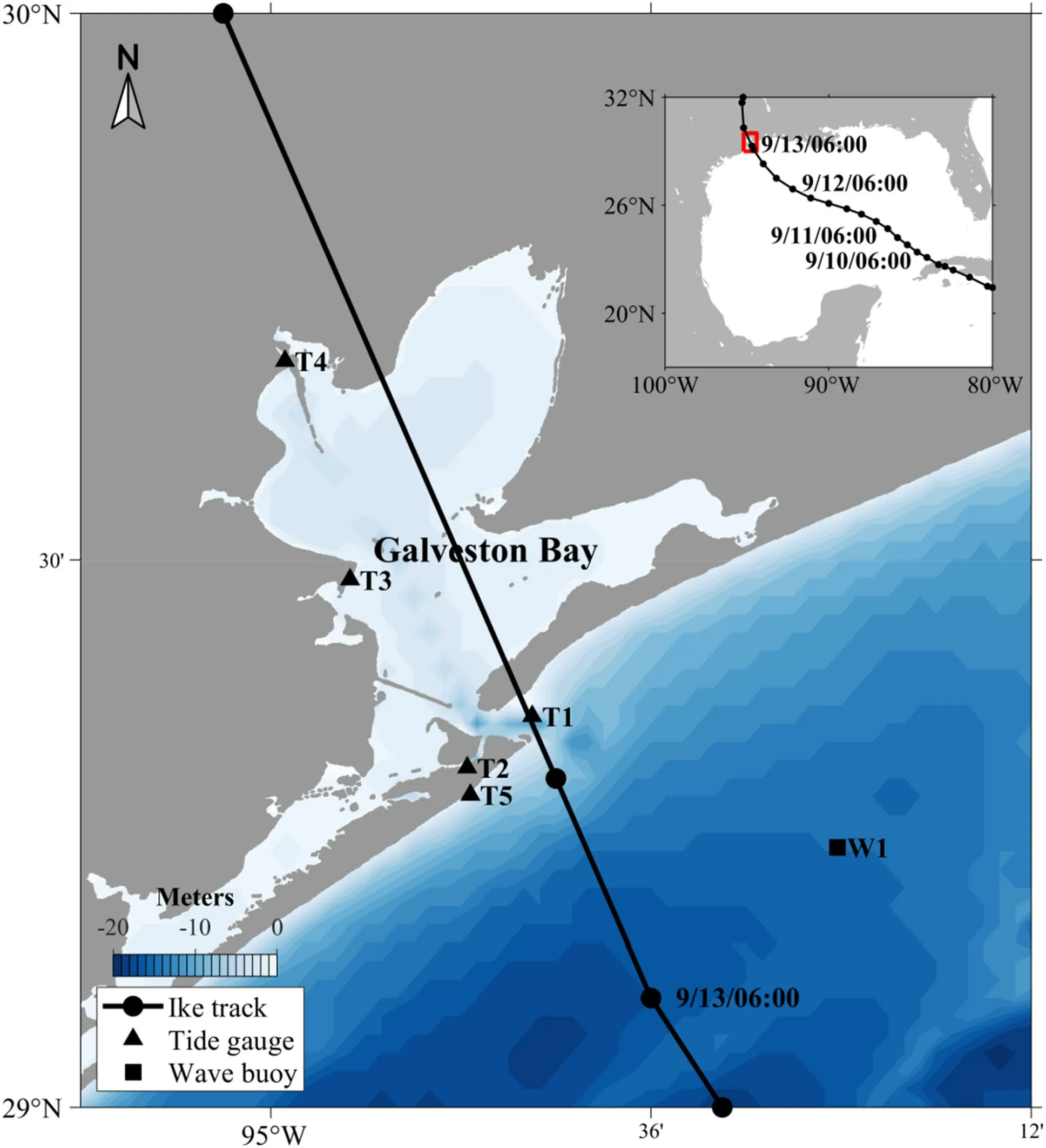
Fig.1 The study area and track of Hurricane Ike.The inset f igure is the Gulf of Mexico, and the red box is the study area, T1–T5 (black triangles) are the tide gauges, and W1 (black square) is the wave buoy.

2.2.1 Data SourcesWe used two topography datasets: a global dataset for the bathymetry (GEBCO2022, 15-arc seconds) for the deep sea,and a high-resolution bathymetry (ETOPO2022, 1-arc second) for Galveston Bay and inland.Astronomical tides (K1,O1, Q1, P1, M2, S2, N2, and K2) on the open boundaries applied harmonics from the OTIS regional and global tidal models (Egbert and Erofeeva 2002).To study the impact of f looding overland, the land roughness was represented in the model with Manning coef ficients.Coef ficient values are based on the land cover classif ications obtained from the 2019 National Land Cover Database (NLCD).1https:// doi.org/ 10.5066/ P9KZC M54.The land cover classif ications were transformed into the corresponding Manning’s n values based on Bunya et al.( 2010).The hurricane track data used in this study were obtained from the Atlantic Hurricane database (HURDAT2), which contains the time, latitude, longitude, central minimum pressure, and central maximum wind speed of the hurricane eye(Franklin and Landsea 2013).The radius to maximum winds from the Tropical Cyclone Extended Best Track Dataset(EBTRK) (Demuth et al.2006) supplemented this dataset.Measured water level, signif icant wave height, wave peak period, wind speed, and pressure values used in the model validation of this study are all from NOAA Tides and Currents.2https:// tides andcu rrents.noaa.gov/.We used more than 20,000 f lood damage claims from the NFIP during Hurricane Ike.These data were obtained from the Institute for a Disaster Resilient Texas and include the number of stories, elevated building indicator, building claim payment, replacement cost, latitude, and longitude of each claim.The model input f iles can be downloaded at http:// deepb lue.lib.umich.edu/ data/ conce rn/ data_ sets/ 8049g 586z.

2.2.2 Hurricane ModelThe accuracy of the simulated storm surge model is primarily contingent upon the precision of external forcing factors,particularly the wind f ield and the reduction in barometric pressure.Delft3D Wind Enhanced Scheme (WES), an integrated module within the Delft3D, utilizes the Holland formula (Holland 2008; Holland et al.2010) and the radius of maximum winds relation formula (Nederhof f et al.2019)based on hurricane data (the HURDAT2 hurricane database was used in this study) to produce wind and air pressure f ields for each hurricane.It is capable of generating hurricane wind and pressure f ields around the storm eye positions on a high-resolution grid.Delft3D WES incorporates asymmetry by taking into account the translational speed of the cyclone center’s displacement by the steering f low, as well as the rotation of wind velocity due to friction (Takagi and Wu 2016).The Delft3D WES output is appropriate for utilization as input in the D-Flow FM model, enabling the simulation of f low and wave patterns, as well as the impact of storm surges.The wind and pressure f ields generated by WES were validated against observations from a NOAA tidal station in Galveston Bay (Fig.1, T3).Three accuracy indicators: the root mean square error (RMSE, Eq.1), the relative root square error (RRSE, Eq.2), and the Pearson correlation coef ficient (＆#x1d70c;, Eq.3) are assessed to validate the model.

wherey′is the model result,yis the observation data and↼yis the average of the observation data,Tis the number of data points, and＆#x1d70e;indicates the standard deviation.The model results for wind speed exhibited strong agreement with the observation data; RMSE, RRSE, and＆#x1d70c;are 5.6 m/s, 0.83, and 0.84 respectively.The model pressure f ield also displayed a robust correlation with the observed data; RMSE, RRSE,and＆#x1d70c;are 3.3 hPa, 0.31, and 0.97 respectively (Fig.2).

2.2.3 Flow and Wave Model Setup

Delft3D Flexible Mesh suite model solves the nonlinear shallow water equations for unsteady f low derived from the three-dimensional Navier-Stokes equations for incompressible free surface f low (Deltares 2022a).A dynamic time step is adopted whereby the model specif ies the time step for each computational step to help maintain model stability and performance in this model.It also integrates the third generation wave model Simulating WAves Nearshore (SWAN), which is a spectral wave model used to solve the wave action balance equation.Delft3D can simulate tidal circulation and the propagation of storm surges in intricate coastal settings and is extensively applied in the modeling of f low and waves during hurricanes (Veeramony et al.2016; Zou et al.2020;Ke et al.2021; Diaz-Loaiza et al.2022; Xu, Tian et al.2022;Al-Attabi et al.2023).

The domain of the f low model covers the northwest of the Gulf of Mexico, roughly ranging from 2ׄ2°N to 32°N and− 98°W to − 86°W (Fig.3 a, b).The grid is further resolved to a grid resolution of about 100 m landward of a line about 5 km of fshore, extending to the western part of Galveston Bay, and consists of 180,000 cells.We used a high-resolution bathymetry of 1 arc-second in Galveston Bay and 15 arc-seconds in other regions.We added a 6 m high f ixed weir (when the water level exceeds 6 m, the seawater can overf low this f ixed weir and f lood the land behind it) in the northeastern part of Texas City to represent a seawall in this region.Astronomical tides on the open boundaries applied harmonics from the OSU Tidal Inversion Software (OTIS)regional and local tidal models.A spatially varying Manning’s coef ficient derived from NLCD was applied to this model.The hurricane model calculated from WES acts as an external force to the model.The wind drag coef ficients used in this model are from Makin ( 2005).The simulation was carried out for a period from 7 to 17 September 2008,the time step ranges from 1 s to 30 s and the other settings are kept as default.

The grids of the wave model are different from the f low model, using structured grids.There are three nesting domains in the wave model.The resolution of the large domain is about 5 km, covering the same spatial extent as the f low domain; the middle domain has a resolution of about 600 m, and covers the whole of Galveston Bay; there are three small domains, each of which has a resolution of about 100 m, and together cover the western part of Galveston Bay (Fig.3 c, d).The wave model grids consist of 201 × 151 cells in the large domain, 124 × 144 cells in the middle domain, and 251 × 201 cells, 171 × 201 cells, and 501 × 71 cells in the small domains.The time step is 60 min.The simulation mode is non-stationary.All the other settingsof the wave model are kept as default (Deltares 2022b) and integrated with the f low model online.Flow and wave simulations exchange data every 60 min via a communication f ile, and the other input data are identical to those used in the f low model.

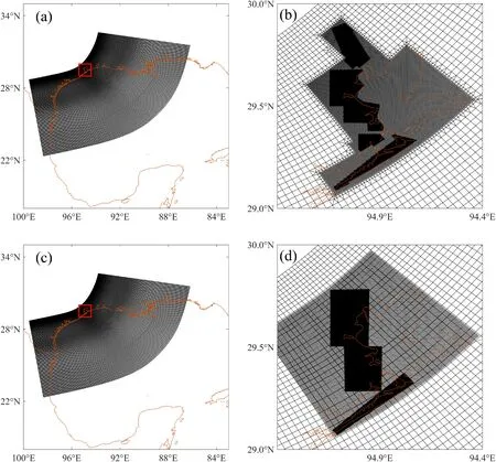
Fig.3 Combination of triangular and curvilinear grids for the f low model and nested computational grid for the wave model.a The overall schematic of the grid, the red box is the study area where the grid is ref ined; b the ref ined area; c the coarse wave grid; d the middle and f ine wave grid

2.2.4 Flow and Wave Model ValidationWe verif ied the accuracy of the integrated model from four aspects: f low water depth, wave height, peak wave period, and inundation water depth.Storm tide is validated against hourly water level data from NOAA tide gauges.Figure 4 shows good agreement between the observed and modeled water levels at T1–T5 (see tide gauge locations in Fig.1) and the RMSE,RRSE, and＆#x1d70c;in Table 1 also indicate that they f it well.The wave model was validated against hourly signif icant wave heights and peak wave period from the NOAA wave buoy W1(Fig.4), and the observed and modeled values also f it well, as shown in Table 1.Assessment of the inundation in Galveston Bay is predominantly qualitative due to the lack of quantitative measurements of f lood depth.An estimate of the observed inundation depth, presented by the Harris County Flood Control District (HCFCD 2009), is illustrated in Fig.5 a; the coast of Galveston Bay shows varying degrees of inundation.Figure 5 b shows the simulated inundation, which can be seen to be consistent with the Harris County Flood Control District map.In summary, our model can simulate Hurricane Ike well.

2.3 Damage Curves

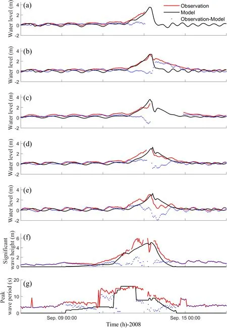
Fig.4 Modeled versus observed water level, signif icant wave height, and peak wave period during Hurricane Ike.a Tide gauge T1 (8771341); b T2(8771450); c T3 (8771013); d T4 (8770613); e T5 (8771510);f signif icant wave height and g peak wave period at buoy station W1 (42035)

whereP(x) is the cumulative probability of the DR with values between 0 and 1,xis the hydrodynamic parameter,Next, we present the extracted maximum values of hydrodynamic parameters on land and the constructed damage curves using both sets of data.Additionally, this section discusses the ef fect of building elevation and number of f loors on the damage curves.

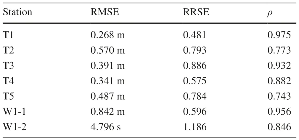
Table 1 Goodness of f it for water level and wave measurements compared with the results of the model

3.1 The Spatial Distribution of DR

The amount of building damage and replacement values for insured structures for western Galveston Bay from the 2008 hurricane Ike event were compiled by the NFIP and were used to calculate DR.From the histogram of DR (Fig.6), about 20% of the structures had a DR higher than 0.5 (considerable damages), 20% had DR between＆#x1d706;is the scale parameter, and＆#x1d705;is the shape parameter.In this study, the function parameters were assessed using the MATLAB Distribution Fitter application.This approach enables the establishment of a relationship between various hydrodynamic parameters and DR.

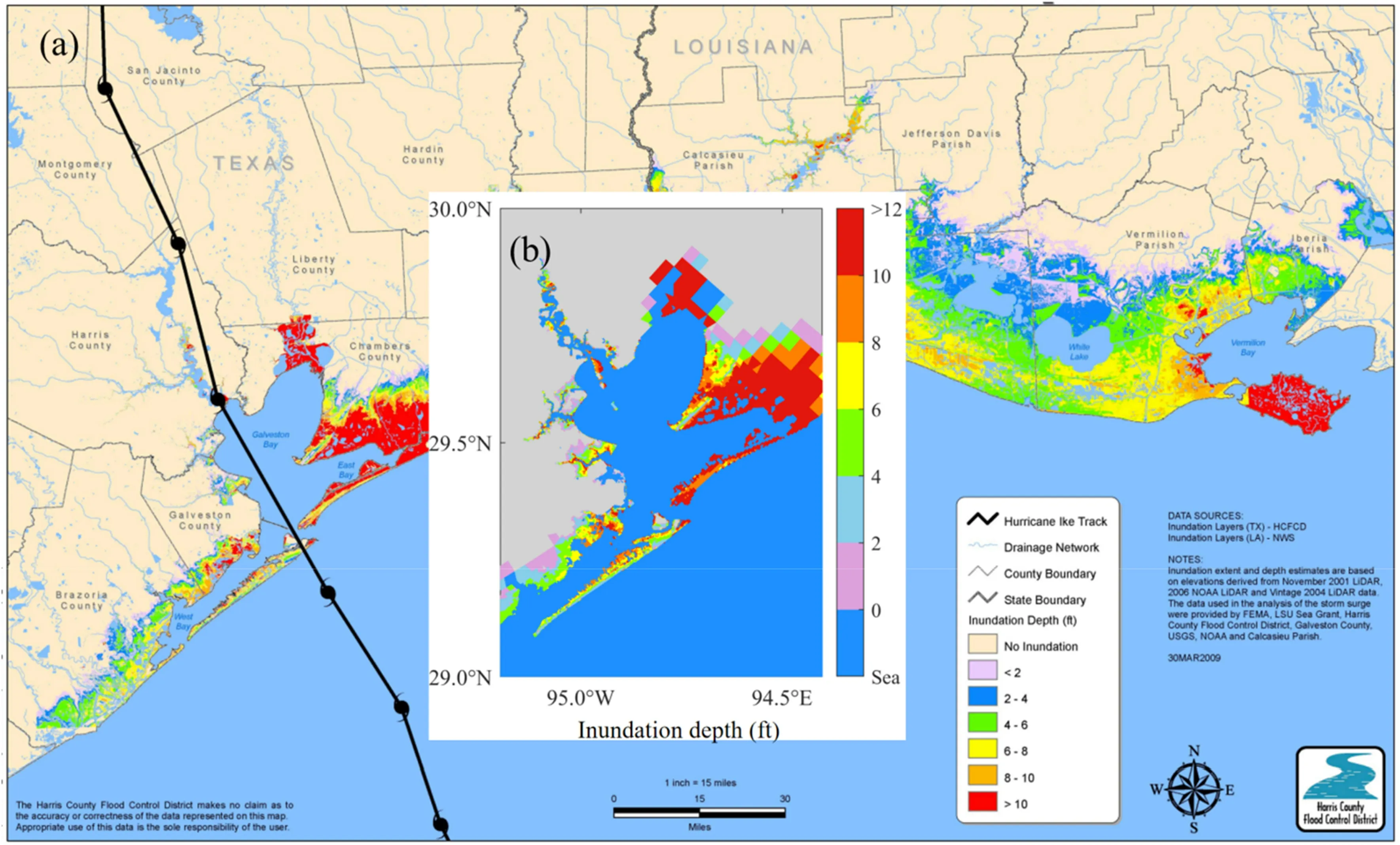
Fig.5 Modeled versus observed inundation depth (ft) during Hurricane Ike.a Observed inundation depth, image from HCFCD ( 2009); b modeled maximum inundation depth

3 Results

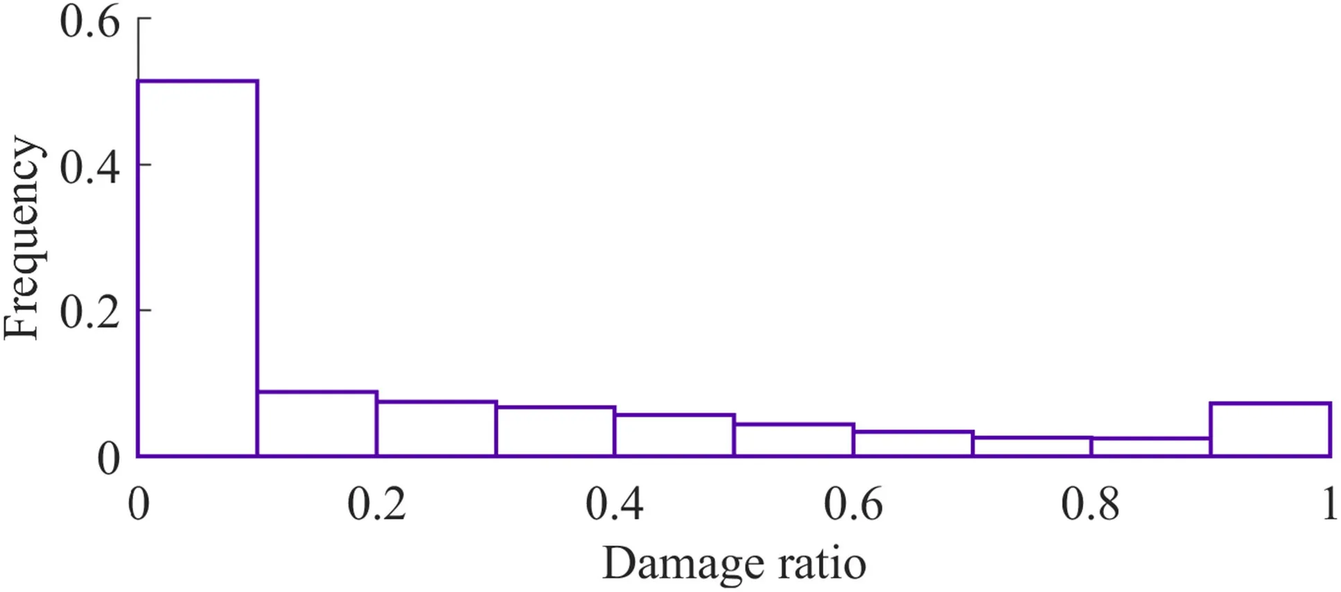
Fig.6 Damage ratio histogram for insurance claims data in the western Galveston Bay region

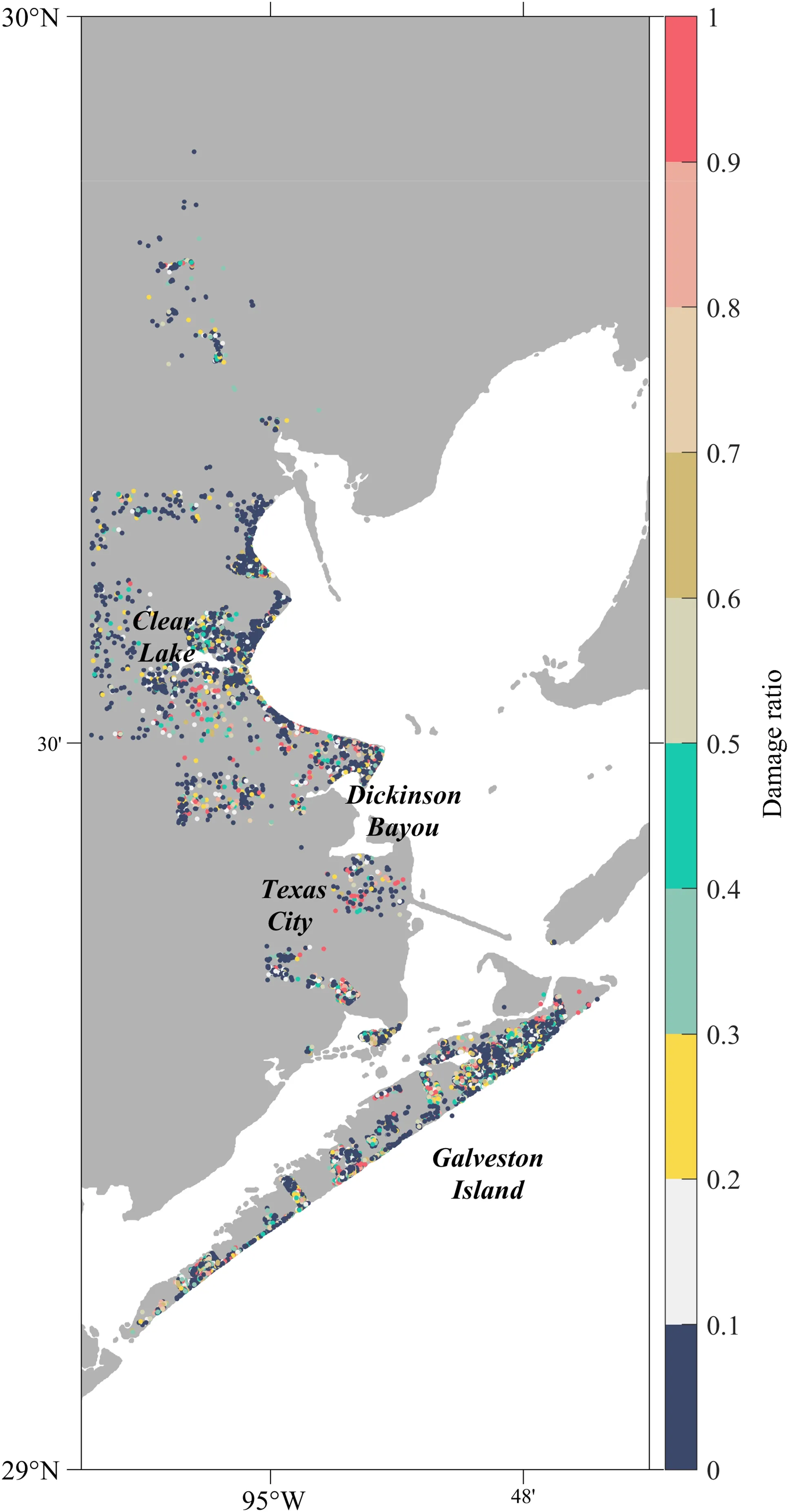
Fig.7 Spatial distribution of DR in the western Galveston Bay region

This study aimed to establish damage curves linking hydrodynamic parameters with DR.In this section, we f irst present the results of calculating DR using NFIP data.0.2 and 0.5 (medium damage), and 60% had low damage (DR < 0.2).This is a typical distribution for damage claims (see for example Fuchs et al.( 2019), Diaz-Loaiza et al.( 2022)).From the spatial distribution of DR (Fig.7),Galveston Island has high DR, followed by Clear Lake,and lower in Texas City and the northwest side of Galveston Bay.

3.2 Maximum Value of Each Hydrodynamic Parameter

After successfully obtained the DR data, we acquired the hydrodynamic parameter data.The water depth, velocity,and signif icant wave height were from the model directly,and unit discharge, f low momentum f lux, total water depth,wave energy f lux, and total force were calculated based on these three parameters (Bricker et al.2017; Diaz-Loaiza et al.2022).We then extracted the maximum values of these hydrodynamic parameters at each grid cell during Hurricane Ike (Fig.8).The entire Galveston Bay largely suf fers from varying degrees of seawater inundation, with the highest levels on the Bolivar Peninsula and Chambers County on the east side.There are f ive main areas of western Galveston Bay that are signif icantly af fected.The entire Galveston Island on the southwest side is f looded and with the strongest hydrodynamic forces of the entire western area, followed by the mainland opposite Galveston Island.The Dickinson Bayou and Clear Lake coastal areas on the west also have strong hydrodynamic forces and most of the coastal areas are f looded.The northwestern bayou area has weaker hydrodynamic forces, with fewer areas f looded.

3.3 Damage Curves from Each Hydrodynamic Parameter

After determining the model f low and wave results at the location of each claim, we analyzed the relationship between the hydrodynamic data and DR data for each claim location to generate damage curves.There is a common method to build damage curves: group DR by hydrodynamic data and then use the cumulative frequency distribution function in Sect.2.3 to f it to obtain the f inal damage curves (Suppasri et al.2013; Tomiczek et al.2017).Suppasri et al.( 2013)used damage data grouped by water depth in building the damage curves during the 2011 tsunami in Japan, and the f it was good.We adopted this method and grouped the DR data according to water depth (0.3 m intervals), f low velocity (0.1 m/s intervals), unit discharge (1 m 2 /s intervals), f low momentum f lux (1 kg/s 2 intervals), signif icant wave height(0.1 m intervals), total water depth (0.5 m intervals), wave energy f lux (50 kW/m intervals), and total force (50 N/m intervals) respectively.The relationship between hydrodynamic data and DR can be seen from the black dots in Fig.9,where the DR gradually increases with the severity of the hydrodynamic hazard.

A comparison to three other typical distribution functions (normal, gamma, and log-normal) was also carried out (Fig.9).It can be seen from Table 2 that the Weibull,normal, and gamma distributions have similar goodness-off it indicators, while the log-normal distribution performs slightly worse overall.Finally, combined with the f itted damage curves in Fig.9, the Weibull distribution function f its better when the DR is below 0.7–0.8 and outperforms the normal and gamma functions overall.Therefore, the results of the f itted damage curves of the Weibull distribution function were used in the subsequent analysis of this study.We found that more than 50% of the damage occurs in the f irst 1.5 m of f lood depth and more than 90% of the damage occurs in the f irst 3 m of f lood depth, which is similar to previous studies (Ruangrassamee et al.2006; Reese and Ramsay 2010; Suppasri et al.2013; Diaz-Loaiza et al.2022).

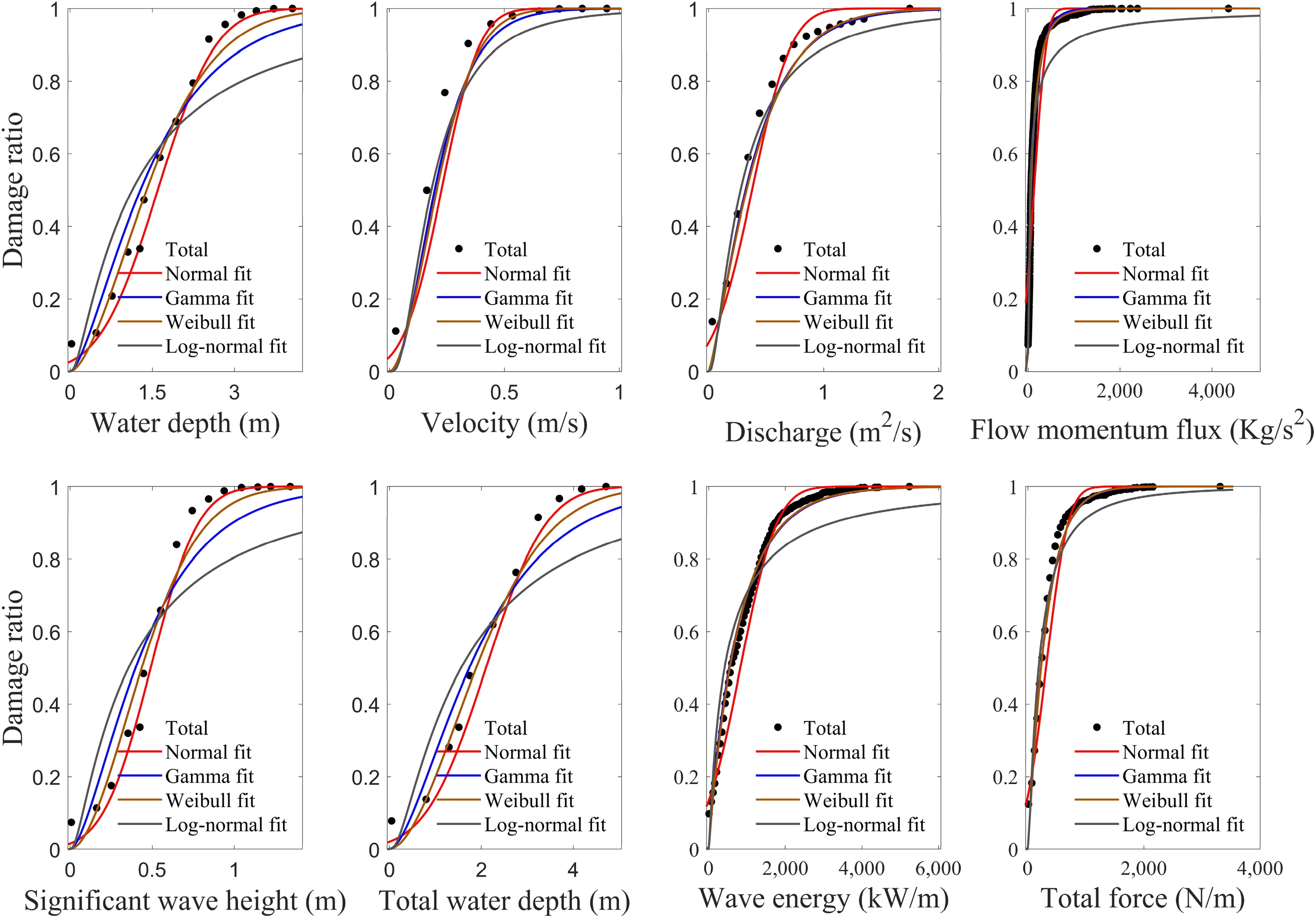
Fig.9 Damage curves for each hydrodynamic parameter

Table 2 Goodness-of-fi t indices for the normal, gamma, Weibull, and log-normal statistical distributions

3.4 Ef fect of Number of Stories and Building Elevation

Pile-elevated coastal residences are common along Galveston Bay, and a study by Tomiczek et al.( 2013) showed a strong inf luence of structural elevation on the damage to coastal residences.Meanwhile, the design of load bearing elements of residential construction dif fers for dif ferent numbers of stories; therefore, the number of stories also af fects the resistance of the building to external forcing(Suppasri et al.2013).The NFIP database reports whether or not buildings are elevated, and whether each building has 1, 2, or 3 or more stories.We therefore divided the NFIP data into six groups: 1 story elevated, 2 stories elevated, 3 stories elevated, 1 story not elevated, 2 stories not elevated,and 3 stories not elevated, and then built the damage curves for these six groups according to the method in Sect.3.3.Figure 10 shows that, except for total water depth, the other seven hydrodynamic parameters had the same trend.For the elevated buildings, the damage curves gradually shift downward with an increase in the number of stories, while the non-elevated buildings have the opposite trend, and these damage curves gradually shift upward with an increase in the number of stories.The damage curves of elevated buildings of three stories and above are the lowest, while the damage curves of non-elevated buildings of three stories and above are the highest, and the damages are the most serious.The damage curves of the other four groups show less dif ference, are located between the f irst two damage curves, and have similar trends.

4 Discussion

In this section, we analyze how damage curves respond to model resolution, discuss their characteristics, compare them with similar damage curves worldwide, and assess their policy implications.

4.1 Sensitivity of Damage Curves to Model Resolution

The resolution of topographic data has been shown to have a signif icant impact on hydrodynamic results and the f itting of damage curves (Veeramony et al.2017; Diaz-Loaiza et al.2022).The grid resolution also has an impact on the results of the model, and a suitable grid resolutionneeds to be selected for the simulation (Al-Attabi et al.2023).Inspired by this, sensitivity tests were conducted to analyze the ef fect of dif ferent grid resolutions on the f itting of damage curves in this study.We designed four grid resolutions (50 m, 100 m, 200 m, and 400 m) to analyze the relationship between water depth and DR, taking water depth as an example.As shown in Fig.11, starting from 400 m, the damage curve gradually shifts upward as the grid resolution increases.When the grid resolution reaches 50 m, the result is almost equivalent to 100 m resolution.This is because the claim locations are located on land, but when the grid resolution is coarse, some claim locations on the shoreline (such as beach houses) are simulated as in the sea, so the modeled hazards at these claim locations are outliers and are not counted in the statistics.Meanwhile, from the results of Sect.3.1, we know that this shoreline region contained many locations with high DR.In summary, the low-resolution grid ignores some claim locations with high DR, resulting in a lower damage curve.Given that the 100 m grid accurately represented the main topographical features, such as shoreline location and navigation channels, increasing the resolution to 50 m did not meaningfully alter the results of the damage curves.However, this increase in resolution substantially increased computational expense.Therefore, in this study,the grid resolution of the study area is set at 100 m.

Fig.10 Damage curves for each hydrodynamic parameter, discriminating based on elevation and number of stories

Fig.11 Damage curves as a function of water depth, with dif ferent grid resolutions

4.2 Analysis of the Damage Curve

Fewer residential structures in northeast Texas City suffered damage (Fig.7), but this area along the coast was not af fected by a strong inundation during the hurricane due to its coastal revetment, which is like a f ixed weir (Fig.8).In Sect.3.4 we can see that a building elevation has a signif icant impact on the ability of the building to resist damage.The non-elevated buildings experienced more damage as the number of stories increased, probably because the DR in this study was derived from the NFIP insurance database determined by the replacement cost of the building, and higher buildings cost more to (re)build than lower buildings.During a hurricane of this magnitude, most of the western Galveston Bay coastal area was inundated by 0.6–3.6 m of water(Fig.8 a), which is already at a depth that has been seen to cause moderate to severe damage (Ruangrassamee et al.2006; Suppasri et al.2013; Fuchs et al.2019; Diaz-Loaiza et al.2022).Non-elevated buildings are af fected by hydrodynamic forces and the impact of f loating debris, incurring higher repair costs.Elevated buildings are relatively less af fected by hydrodynamic forces due to their distance from the ground, and the required repair costs are lower than those of non-elevated buildings when the strong resistance of multiple stories is more prominent.Thus, elevated buildings experience less damage as the number of stories increases.Also, the overall damage curves of elevated buildings are lower than that of non-elevated buildings.

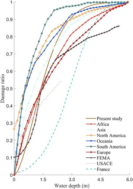
Fig.12 Comparison of damage curves for water depth in dif ferent regions of the world.The data of Africa, Asia, North America, Oceania, South America, and Europe are from Huizinga et al.( 2017);FEMA data are from Tomiczek et al.( 2013); USACE data are from Wing et al.( 2020); France data are from Diaz-Loaiza et al.( 2022).

It is well-documented that insurance claims can be susceptible to fraud or misinformation (Diaz-Loaiza et al.2022).Furthermore, factors related to asset vulnerability,such as construction characteristics, materials used, quality, and structure age (Suppasri et al.2013; Paprotny et al.2020), play crucial roles in determining the extent to which a specif ic hydrodynamic variable is associated with damage.This introduces an additional layer of complexity to the analysis.Moreover, it is noteworthy that if more detailed information from the claims data were accessible, such as structure type, structure age, and damage stage, it would enable the generation of more intricate fragility functions.Finally, the maximum limit of the NFIP coverage is up to USD 250,000 for buildings and USD 100,000 for content(Kousky 2018).Hence, the dollar amount of building claim(a measure of loss) may be underreporting sustained structural damages for buildings with the value exceeding USD 250,000.More accurate damage assessment at the structure level will certainly improve the reliability of damage curve estimates.

4.3 Comparison with Other Global Damage Curves

A comparison of building damage curves with previous f indings can be made using water depth as an example.A summary of building damage curves from many locations (Tomiczek et al.2013; Huizinga et al.2017; Wing et al.2020; Diaz-Loaiza et al.2022) is shown in Fig.12.The damage curve in Galveston Bay is characterized by two regions compared to other damage curves.When the water depth is below about 1.5 m, the damage curve in this area is lower than most of the others.When the water depth exceeds 1.5 m, the slope of the Galveston Bay damage curve increases sharply.DR exceeds 90% at about 3 m.This is because when the water depth is low,this region has a lower DR than other regions of the world due to the presence of elevated buildings.

4.4 Policy Implications

This study has highlighted the importance of structural elevation for coastal hazard mitigation as the overall damage curves of elevated buildings are found to be lower than that of non-elevated buildings.Structural elevation requirements are tied to standards put forth by the NFIP to protect against a 1%-annual-chance f lood or 100-year f lood.Location-specif ic base f lood elevation requirements (BFE), designated by FEMA Flood Insurance Rate Maps (FIRMs), are the minimum standard for elevation of new, substantially damaged, or improved structure construction.Communities are encouraged to set elevation requirements above the BFE standards, and certain classes of Community Rating System communities, working to receive credit toward discounted f lood insurance premiums,must adopt freeboard requirements above the BFE (FEMA 2020).Elevation above NFIP 100-year f loodplain requirements is increasingly important as extreme weather events and studies have revealed f looding outside of the 100-year f loodplain(Brody and Highf ield 2011; Highf ield et al.2013; Brody et al.2014; Blessing et al.2017; Rainey et al.2021), and climate change is intensifying heavy precipitation events (Tabari 2020).Research has long established that f lood damage is decreased with adoption of freeboard standards (Godschalk et al.1989; Highf ield et al.2014), and coastal residents have been found to be supportive of elevation.In a study of Upper Texas coastal residents, including those of Galveston Island,Ross and Atoba ( 2022) found that structural elevation is the most supported hazard mitigation strategy with 65% of the survey respondents saying they “support a lot” this strategy.The issue in widespread policy adoption of higher standards for elevation, therefore, is improved knowledge of future climate risk to determine just how high structures should be.Current f loodplain maps and elevation standards are based on historic data; they do not factor in sea level rise and changing climate conditions (Pralle 2019).Updates to NFIP risk rating methodology are making only incremental improvements by including additional (historic) f lood variables (FEMA n.d.).Until f lood maps account for future f lood risk, minimum elevation standards will fail to provide the protection needed (Pralle 2019).observations conf irm that the model performed ef fectively in hindcasting the f low and wave processes during this event.We then generated damage curves for this region using eight modeled hydrodynamic parameters and DRs derived from NFIP data using the Weibull cumulative distribution function.We have thus drawn the following conclusions:

• About 50% of the damage occurs in the f irst 1.5 m of f lood depth and about 90% of the damage occurs in the f irst 3 m of f lood depth.

• The damage curve becomes higher as the grid resolution increases, but stabilizes when the resolution reaches 100 m.

• The damage curves of elevated buildings in this area decrease with a greater number of stories and are lower than the damage curves of non-elevated buildings.The damage curves of non-elevated buildings show the opposite trend, increasing with an increase in the number of stories.Therefore, elevated buildings have an important inf luence on the resistance of buildings to damage during hurricanes.

• Compared to other depth-damage functions from the literature, the depth-damage curve for Galveston Bay predicts a lower DR for inundation depth less than 1.5 m,but a higher DR for inundation depth greater than 1.5 m.

The current study considers only monovariate damage curves, applying only 1 forcing variable at a time.Future work can include multivariate damage analysis, investigating the correlation of damage with many forcing variables using machine learning (Nateghi et al.2016).

AcknowledgmentsThis research was funded by NSF award 2228486 under the program Strengthening America’s Infrastructure.Chaoran Xu acknowledges funding from the China Scholarship Council, Grant No.202206140090.

Open AccessThis article is licensed under a Creative Commons Attribution 4.0 International License, which permits use, sharing, adaptation, distribution and reproduction in any medium or format, as long as you give appropriate credit to the original author(s) and the source,provide a link to the Creative Commons licence, and indicate if changes were made.The images or other third party material in this article are included in the article’s Creative Commons licence, unless indicated otherwise in a credit line to the material.If material is not included in the article’s Creative Commons licence and your intended use is not permitted by statutory regulation or exceeds the permitted use, you will need to obtain permission directly from the copyright holder.To view a copy of this licence, visit http://creativecommons.org/licenses/by/4.0/.

5 Conclusion

In this study, we simulated storm surges and waves from Hurricane Ike, which impacted Galveston Bay in September 2008.Comparisons of water level, signif icant wave height,peak wave period, and inundation depth with multiple