Assimilation of Ocean Surface Wind Data by the HY-2B Satellite in GRAPES: Impacts on Analyses and Forecasts

Jincheng WANG, Xingwei JIANG, Xueshun SHEN, Youguang ZHANG,Xiaomin WAN, Wei HAN, and Dan WANG

1CMA Earth System Modeling and Prediction Center, China Meteorological Administration, Beijing 100081, China

2National Meteorology Center, China Meteorological Administration, Beijing 100081, China

3Southern Marine Science and Engineering Guangdong Laboratory (Guangzhou), Guangzhou 511458, China

4National Satellite Ocean Application Service, Beijing 100081, China

ABSTRACT The ocean surface wind (OSW) data retrieved from microwave scatterometers have high spatial accuracy and represent the only wind data assimilated by global numerical models on the ocean surface, thus playing an important role in improving the forecast skills of global medium-range weather prediction models.To improve the forecast skills of the Global/Regional Assimilation and Prediction System Global Forecast System (GRAPES_GFS), the HY-2B OSW data is assimilated into the GRAPES_GFS four-dimensional variational assimilation (4DVAR) system.Then, the impacts of the HY-2B OSW data assimilation on the analyses and forecasts of GRAPES_GFS are analyzed based on one-month assimilation cycle experiments.The results show that after assimilating the HY-2B OSW data, the analysis errors of the wind fields in the lower-middle troposphere (1000-600 hPa) of the tropics and the southern hemisphere (SH) are significantly reduced by an average rate of about 5%.The impacts of the HY-2B OSW data assimilation on the analysis fields of wind, geopotential height, and temperature are not solely limited to the boundary layer but also extend throughout the entire troposphere after about two days of cycling assimilation.Furthermore, assimilating the HY-2B OSW data can significantly improve the forecast skill of wind, geopotential height, and temperature in the troposphere of the tropics and SH.

Key words: HY-2B, ocean surface wind, 4DVAR, GRAPES-GFS, medium-range weather forecast

1.Introduction

The Global Data Assimilation System (GDAS) is one of the core components of the global numerical weather prediction (NWP) system, which provides the initial condition for integrating an NWP model.Presently, two main categories of observational data can be assimilated into the GDAS, 1)conventional observational data, including surface observations, upper-air observations, aircraft-based observations,and ship observations, and 2) observations that are gathered by remote sensing satellites, which are mainly comprised of the brightness temperature data of the polar-orbiting and geostationary satellites, the refractivity data of the Global Navigation Satellite System-Radio Occultation (GNSS-RO), and the cloud-derived wind data retrieved from the polar-orbiting and geostationary satellites.The satellite observations effectively fill the shortage of conventional observational dataover the ocean and thus significantly improve the skill of global numerical weather forecasts.Satellite observations are playing an increasingly important role in promoting the development of today’s NWP (Cardinali, 2009).

Despite a growing amount of satellite observations, the most collected variable by satellite observations is the brightness temperature (mass field).The number of wind (motion field) observations is relatively lower over the ocean, with only the atmospheric motion vectors (AMVs) data available in cloud regions (Feng and Wang, 2019).Because geostrophic balance between the motion field and the mass field is not satisfied in tropical regions, the existing data assimilation algorithm is incapable of deriving the high precision motion field from the observational data of the mass field, which limits the accuracy of the initial condition potentially leading to poor forecasting skill for typhoon and other disastrous weather events in the tropics.To remedy the lack of wind observations over the ocean, the microwave scatterometer was developed to observe the ocean surface wind(OSW) (Figa-Saldaña and Stoffelen, 2000; Figa-Saldaña et al., 2002).Owing to the continuous improvement of the OSW retrieval algorithm, the accuracy of the OSW data is also dramatically enhanced (Hersbach et al., 2007; Wang et al., 2015; De Kloe et al., 2017; Lin et al., 2017a; Wang et al., 2017).The main NWP operational centers across the world have incorporated the assimilation of the OSW data into operation, which greatly improved the forecast skills of global NWP (Ayina et al., 2006; Candy and Keogh, 2006;Hersbach, 2010; Bi et al., 2011; Laloyaux et al., 2016; De Chiara et al., 2016, 2017; Duan et al., 2017).The OSW data assimilated in the GDAS is mainly collected by the advanced scatterometer (ASCAT) onboard the Meteorological Operational Satellite-A/B and the quick scatterometer(QuickSCAT) and the Ku-band scatterometer mounted onboard the HY-2A satellite (HSCAT-A) (Bi et al., 2011;Jiang et al., 2012; De Chiara et al., 2016; Lin et al., 2017b).

The HY-2B satellite is the second ocean dynamic environment monitoring satellite following the HY-2A satellite(Jiang et al., 2013).It was successfully launched on 25 October 2018, equipped with a Ku-band rotating fan-beam scanning scatterometer (HSCAT-B).The HSCAT-B OSW retrieval algorithm is designed based on the mature retrieval algorithm and quality control algorithm of the HY-2A scatterometer (HSCAT-A) (Jiang and Lin, 2009; Wang et al.,2015, 2017; Lin et al., 2017a).The evaluation shows that the OSW of HSCAT-B is clearly more accurate than that of HSCAT-A and has similar precision to that of ASCAT-A/B(Wang et al., 2020).Data retrieved from ASCAT-A and B OSW have displayed good accuracy when assessed with dropwindsonde and buoy winds (Chou et al., 2013; Lin et al.,2015).Many operational centers have assimilated ASCATA and B OSW data into global numerical weather prediction systems operationally (e.g., ECMWF, NCEP), and it has made a significant contribution to improving forecast skill(Bi et al., 2011; De Chiara et al., 2016; Lin et al., 2017b).These assessment results lay a solid foundation for the assimilation and application of HSCAT-B OSW in global numerical weather prediction.Meanwhile, compared with the two small observational swaths (～550 km) of ASCAT,the observational swath of HSCAT-B is as large as 1800 km,which covers 90% of the global ocean area.As a result, the amount of retrieved OSW data is more than 1.5 times that of ASCAT given the same spatial resolution.

So far, studies on the assimilation of the HSCAT-B OSW and its impact on the initial analysis and forecast of NWP model are lacking.Therefore, to investigate the optimal scheme for the processing and assimilation of the HSCATB OSW data and improve the forecast performance of the Global/Regional Assimilation and Prediction System(GRAPES) over oceanic regions, this study designed and carried out a one-month HSCAT-B OSW data assimilation experiment based on the GRAPES global four-dimensional variational assimilation system (4DVAR), and evaluated the influence of the HSCAT-B OSW data on the forecast skills of GRAPES Global Forecast System (GRAPES_GFS).Our results are expected to offer useful insight into applying OSW data from the HSCAT-B and the Chinese-French Oceanography Satellite in the future.

The remainder of this paper is organized as follows.Section 2 discusses the assimilation system and experimental design.Section 3 presents the assimilation data and the results.Section 4 provides a discussion and conclusion.

2.Assimilation system, HSCAT-B ocean surface wind, and experimental design

2.1.GRAPES global four-dimensional variational data assimilation system

The GRAPES global four-dimensional variational data assimilation system (GRAPES_GFS 4DVAR) adopts the incremental analysis update scheme (Zhang et al., 2019).Compared with the three-dimensional variational data assimilation system (3DVAR), the amount of observational data that can be effectively ingested in the 4DVAR system is increased by 50%; consequently, the analysis and forecast error amplitude significantly decreases (Zhang et al., 2019).The assimilation window of GRAPES_GFS 4DVAR is six hours, and the observational time slot is 30 minutes, which means the GRAPES_GFS 4DVAR can assimilate the observational data with high temporal resolution.The assimilated observational data in this study include the conventional observational data and the satellite observational data, as summarized in Table 1.The forecast model used in this study is GRAPES_GFS V3.0, which is currently operated at the China Meteorological Administration with a horizontal resolution of 0.25° × 0.25° with 87 vertical layers.The main physical parameterization schemes in GRAPES_GFS V3.0 are shown in Table 2.The long- and short-wave radiation scheme is generated by the Rapid Radiative Transfer Model(RRTMG) (Morcrette et al., 2008).The land surface scheme used is the Common Land Model (CoLM) (Dai et al., 2003).The planetary boundary layer scheme used is the Medium-Range Forecast (MRF) (Hong and Pan, 1996).The deep and shallow cumulus convection parameterization scheme is given by the New Simplified Arakawa-Schubert (NSAS) subroutine (Arakawa and Schubert, 1974; Pan and Wu, 1995;Liu et al., 2015).The cloud physics schemes include a explicitly prognostic cloud cover scheme (Ma et al., 2018) and the CMA double moment microphysics scheme, the macrophysics cloud condensation scheme, the impacts of detrainment of deep/shallow convection on grid-scale clouds to represent the processes of formation and extinction for all hydrometeros.(Tan et al., 2013; Jiang et al., 2015; Chen et al., 2021).In the incremental 4DVAR, the numbers of vertical layers of inner and outer loops and the horizontal resolution of the outer loop are the same as those in the GRAPES operational model.The horizontal resolution of the inner loop is 1.0° × 1.0°.In GRAPES_GFS 4DVAR, the OSW data is directly assimilated as the 10 m neutral wind over the ocean surface.The deblurred zonal wind component (u) and meridional wind component (v) products of HY-2B are also assimilated.

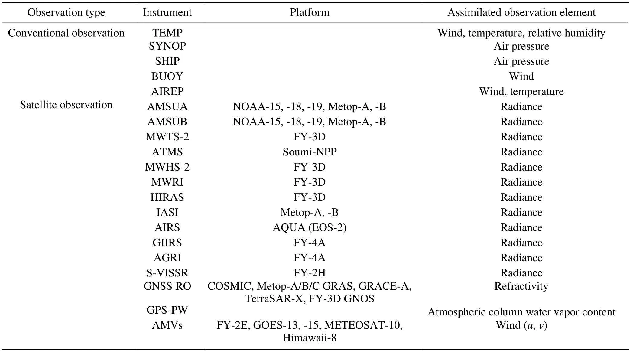
Table 1.Observations and variables assimilated in the control experiment (CTRL).

Table 2.Parameterization schemes for physical processes used in GRAPES_GFS V3.0.

2.2.HSCAT-B ocean surface wind

The HSCAT-B OSW data retrieved by the National Satellite Ocean Application Service (NSOAS) is assimilated in this study, with a horizontal resolution of 25 km.The NWP-based ocean calibration (NOC) algorithm is used for the HSCAT-B OSW retrieval, which considers the influence of sea surface temperature and exerts strict quality control (Verspeek et al., 2012; Wang et al., 2015, 2017; Lin et al.,2017a).The results show that the root mean square errors(RMSEs) of wind speed and wind direction of the HSCATB OSW data after strict quality control are 2.26 m s-1and 16.6°, respectively, evaluated against the buoy wind data.The accuracy of the HSCAT-B OSW data is equivalent to that of the ASCAT-B OSW data (Wang et al., 2020).

2.3.Observational error

With the wind data observed by oceanographic buoys as a reference, the RMSEs of u and v of the HSCAT-B OSW data are 1.70 m s-1and 1.76 m s-1, and the biases are 0.03 m s-1and -0.08 m s-1, respectively (Wang et al., 2020).Although the bias of HSCAT-B is relatively small, previous research showed that the bias is quite sensitive to the actual wind speed.The bias of the HSCAT-B wind speed is particularly obvious when the wind speed becomes larger than 20 m s-1(Wang et al., 2020).However, there is no bias correction procedure especially for the OSW data in GRAPES_GFS.To mitigate the potential influence of the bias, the observational error should be appropriately enlarged.In addition, the spatial resolution of the u and v components of the OSW retrieval is set at 25 km, which is slightly finer than that of GRAPES_GFS.In general, the correlation between the observational errors of adjacent grids within the current resolution of 25 km should be considered.Previous studies also demonstrated that the spatial correlation of ASCAT-B observational errors approaches zero when the grid interval is beyond 50 km (Valkonen et al., 2017).Nonetheless, in GRAPES_GFS 4DVAR assimilation system, the correlation between observational errors of adjacent grids is not considered in the observational error covariance matrix due to computational cost.Therefore, we process the HSCAT-B OSW observations with the thinning step and enlarge the observational errors in the assimilation system to 2 m s-1for the u and v wind components.

2.4.Quality control

There are strict quality controls in the retrieval process of the HSCAT-B OSW (Lin et al., 2017a; Wang et al.,2020).The quality control algorithm for the HSCAT-B OSW L2b products is used to eliminate the data over the areas covered with sea ice and those polluted by precipitation before the GRAPES_GFS 4DVAR assimilation.The quality of observations is controlled by comparing against the background field in GRAPES_GFS 4DVAR.Specifically, the observational data that satisfy the following condition are eliminated:

whereyois the observation of u or v,ybis the background value of u or v, σois the observational error of u or v, andβ is the threshold constant of quality control.In this study, β is set to 9 in the GRAPES_GFS 4DVAR assimilation system.

2.5.Data thinning

There is a significant correlation between the observational errors of the scatterometer-retrieved OSW across adjacent grids, so it is necessary to thin the pre-processed OSW data before being assimilated (Ochotta et al., 2005; Duan et al., 2017; Valkonen et al., 2017).Previous studies have shown that the assimilation result is optimal when the grid interval of OSW data is 100 km (Bi et al., 2011; Valkonen et al., 2017).Therefore, during the data thinning for HSCAT-B OSW, only one out of four adjacent grid observations is assimilated, which forces the generation of the OSW data to have a horizontal resolution of 100 km.

2.6.Experiment design

Table 3 addresses the experimental configurations.The observational data assimilated in the control experiment(CTRL) are the same as those in the operational GRAPES_GFS (Table 1).The conventional observations include radiosonde data, surface observational data, aircraftbased data, ship data, and buoy data.The assimilated satellite data include the radiance data observed by the Advanced Microwave Sounding Unit-A (AMSU-A), the data from the Microwave Humidity Sounder (MHS) over multiple satellite platforms (NOAA15, etc.), the infrared hyperspectral radiance data observed by the Infrared Atmospheric Sounding Interferometer (IASI) of METOP-A and METOP-B, the infrared hyperspectral radiance data observed by the atmospheric infrared sounder (AIRS) of EOS-2, the radiance data observed by the Micro-Wave Humidity Sounder-2(MWHS-2) of FY-3D, the radiance data observed by the Micro-Wave Temperature Sounder-2 (MWTS-2) of FY-3D,the Hyperspectral Infrared Atmospheric Sounder (HIRAS)of FY-3D, the radiance data observed by the Microwave Radiation Imager (MWRI) onboard the FY-3D, the brightness temperature observed by the Geostationary Interferometric Infrared Sounder (GIIRS) and the Advanced Geosynchronous Radiation Imager (AGRI) onboard FY-4A, the radiance data observed by the Stretched Visible and Infrared Spinscan Radiometer (S-VISRR) onboard FY-2H, the refractivity data of navigation satellites (COSMIC, etc.), and the Atmosphere Motion Vectors (AMVs) data of geostationary satellites from multiple satellite platforms (FY-2E, etc.).The HSCAT-B assimilation experiment (HSCAT_EXP) adds the assimilation of HSCAT-B OSW data based on the CTRL.

Table 3.Experimental configurations.

Both experiments have the same assimilation window of six hours and an observational time slot of 30 minutes.The one-month experimental period spans 1 September to 30 September 2020, with a total of 120 data assimilation(DA) and forecast cases.

3.The assimilation effect of the HACAT-B OSW data

3.1.Influence of assimilating HSCAT-B OSW on the analysis

Figure 1 shows the distribution of the probability density function of the difference between the HSCAT-B OSW observations and the background field (i.e., observation minus background, OMB, and also termed the innovation vector).The difference between the observations and the analysis fields (i.e., observation minus analysis, OMA, also termed the residual) is also given.It shows that the probability density functions of OMB and OMA for u and v of HSCAT-B are very close to a normal distribution.The mean values of OMA and OMB are very close, while the standard deviation of the former is significantly smaller than that of the latter(1.212 m s-1vs.1.604 m s-1for u and 1.207 m s-1vs.1.598 m s-1for v).The results indicate that the probability density function of OMB is very close to a Gaussian distribution, which meets the requirement of the variational assimilation.Moreover, the evidently smaller standard deviation of OMA compared to OMB indicates the effectiveness of assimilating HSCAT-B OSW data in GRAPES_GFS 4DVAR.

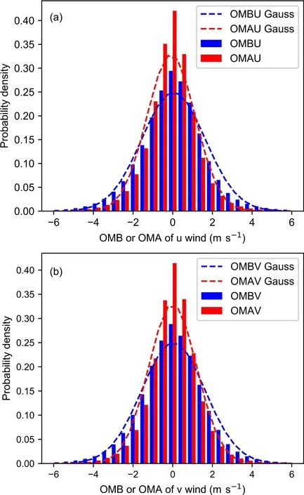
Fig.1.The probability density function distribution (histogram) of the OMB(blue) and the OMA (red), and the Gaussian distribution (dotted line) with the same means and standard deviations as OMB and OMA, for the HSCAT-B (a)zonal wind, u and (b) meridional wind, v.

Figure 2 shows the number of the assimilated HSCATB wind observations within each grid box (i.e., a 2.5° by 2.5°box) and the mean and standard deviation of the OMB and OMA calculated for all the observations with each grid box.The spatial distribution of the number of the assimilated HSCAT-B wind data in HSCAT_EXP (Fig.2a) displays obvious satellite orbital characteristics, and there are four zones with high number values at longitudes of 45°E, 135°E,45°W, and 135°W.In addition, there is a high-value area over the Arctic Ocean (north of 60°N).Figure 2b shows the mean OMB of u.Compared with the HSCAT-B observations, the background field of GRAPES_GFS has an obvious westerly wind deviation in the middle latitudes (30°-60°N,30°-60°S) and an overall easterly wind deviation in the tropical regions.It also shows a westerly wind deviation in the core areas of El Niño-Southern Oscillation (ENSO) and the coastal areas of the main continents (such as the east, south,and west coasts of Africa and the coast of Eurasia).After the HSCAT-B u-wind is assimilated, the analysis of the deviation of the u-wind (Fig.2c) is significantly reduced relative to the background field.As for the v-wind in Fig.2d, there is an obvious southerly wind deviation in the northern hemisphere and a northerly wind deviation in the southern hemisphere.This implies a net deviation of mass transport from the equator to the two poles in the lower levels of GRAPES_GFS.After the HSCAT-B wind field is assimilated, the deviation of the v-wind is also significantly reduced (Fig.2e).Figures 2f and 2h are the standard deviations of the OMB of u and v, respectively.The results show that the horizontal distribution patterns of the standard deviations of the OMB of u and v are very similar.The standard deviations are relatively large in the inter-tropical convergence zone (ITCZ) and the high latitude zones.Figures 2g and 2i show the OMA standard deviations of u and v, respectively.Compared with the OMB standard deviations of u(Fig.2f) and v (Fig.2h), the OMA standard deviations of u and v are significantly reduced.The comparison results of OMB and OMA in Figs.1 and 2 indicate that the information of the HSCAT-B OSW data has been effectively ingested into the GRAPES_GFS 4DVAR analysis.

To evaluate the impact of the assimilation of HSCAT-B OSW data on the analysis fields of GRAPES_GFS, the ERA-Interim reanalysis data is used as the reference field to calculate the RMSE of a given variable (denoted by x) in the analysis fields of both the CTRL and HSCAT_EXP experiments.

Figures 3a-d are the RMSEs of u, v, geopotential height, and temperature in the analysis fields, respectively.The comparison between HSCAT_EXP and CTRL shows that the RMSE of wind in the lower levels (below 600 hPa)decreases significantly in all three regions after assimilating the HSCAT-B OSW data, especially in the tropics and southern hemisphere.The improvement in the geopotential height field is qualitatively similar to the wind field, as the geostrophic component is physically related to the wind.However, the RMSE of temperature demonstrates little change in the two experiments.The results indicate that the influence of the HSCAT-B data assimilation is mainly on the momentum variables in analysis fields below 600 hPa, namely the atmospheric boundary layer (ABL) and the lower troposphere.

To further analyze the influence of the HSCAT-B OSW data assimilation on different levels of analysis fields, the reduction rate of RMSE in the HSCAT_EXP experiment to that in the CTRL experiment at each analysis time (%) is calculated as follows:

The mean reduction rate of RMSE at multiple analysis times is calculated as the following:

wherePis the number of analysis cycles.

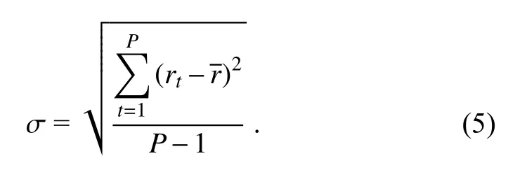
The standard deviation of the RMSE reduction rate is calculated as follows:

The average reduction rates of RMSEs for each variable in the analysis fields of HSCAT_EXP are presented in Fig.4.Figures 4a-b show that, after assimilating the HSCAT-B OSW data, the RMSEs of u and v within 1000-600 hPa are reduced with an average reduction rate of about 5%, significant at the 0.01 level.The average reduction rate of RMSE is largest for the southern hemisphere, followed by tropical regions and the northern hemisphere.The RMSE reduction rate decreases with increasing height and approaches zero at near 600 hPa.The above results indicate that the assimilation of the HSCAT-B OSW data can significantly reduce the analysis errors of u and v in the ABL and the lower troposphere.

In terms of the geopotential height, the RMSE of the analysis of HSCAT_EXP is 2%-9% lower than that of CTRL within the whole troposphere (Fig.4c).The reduction rate is

largest near the surface (～1000 hPa).The RMSE reduction rates of geopotential height at 1000 hPa are 6%, 9%, and 3%in the southern hemisphere, northern hemisphere, and tropics, respectively.The uncertainty range in Fig.4c indicates that the RMSE reduction rate of the geopotential height is significant at 1000-500 hPa for the southern hemisphere and the tropics, while it is significant only for the near-surface layer (below 925 hPa) in the northern hemisphere.

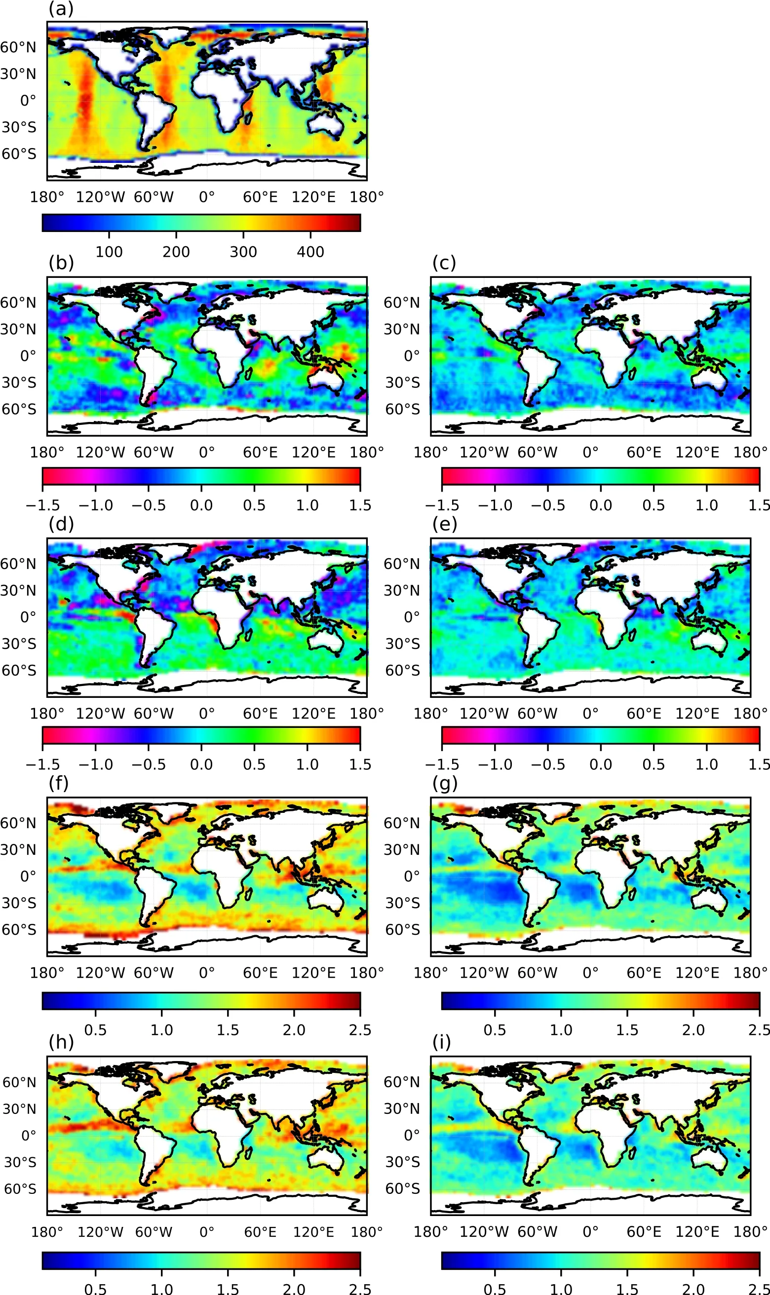
Fig.2.The means and standard deviations of the OMA and OMB of the HSCAT-B winds assimilated on a 2.5° by 2.5° grid.(a) The count, (b) the OMB mean of u, (c) the OMA mean of u, (d) the OMB mean of v, (e) the OMA mean of v, (f) the OMB standard deviation of u, (g) the OMA standard deviation of u, (h) the OMB standard deviation of v, and (i) the OMA standard deviation of v.

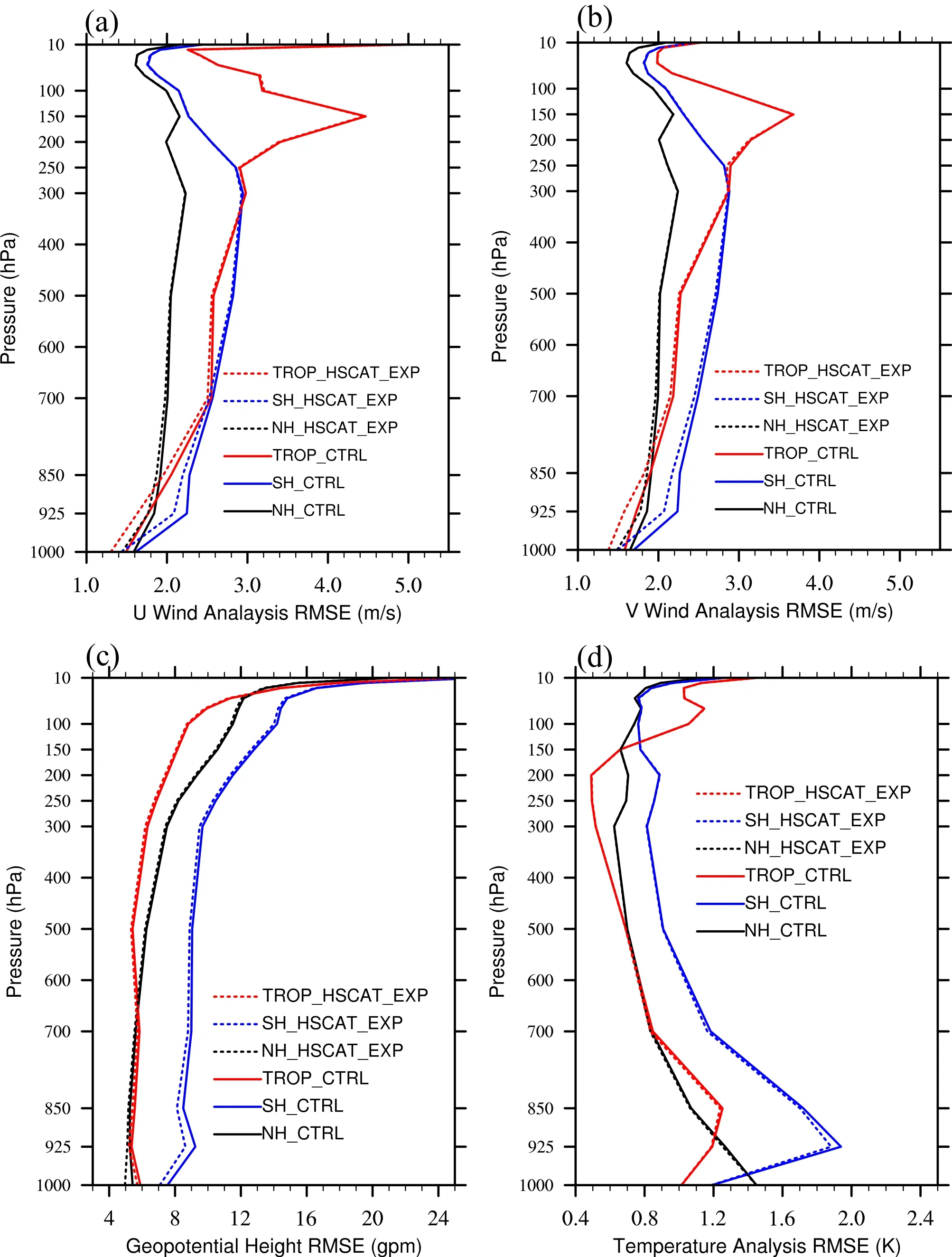
Fig.3.The average analysis RMSEs in the southern hemisphere (blue line), northern hemisphere (black line), and tropical regions(red line) for the CTRL (solid line) and HSCAT_EXP (dashed line) experiments for the (a) zonal wind, (b) meridional wind, (c)geopotential height, and (d) temperature.

Different from the wind and geopotential height, the maximum RMSE reduction rate for temperature is located within 925-500 hPa (Fig.4d).The RMSE reduction is significant at nearly 950 hPa in the southern hemisphere, though the RMSE reduction rate is small overall, with an average rate of less than 1%.

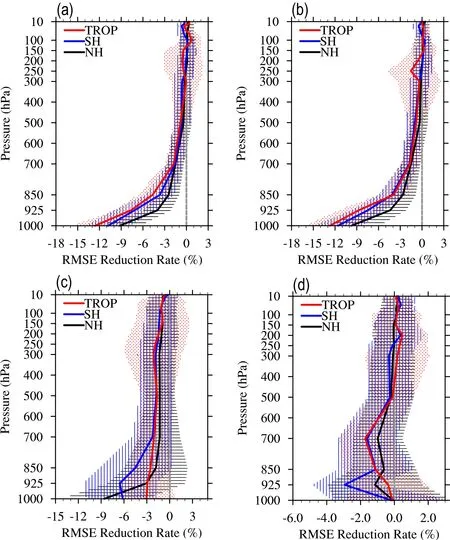
Fig.4.The average reduction rates (units: %) of RMSE of the (a) zonal wind, (b) meridional wind, (c) geopotential height, and (d) temperature of the HSCAT-EXP experiment in September 2020.The black and blue solid lines represent the northern hemisphere and southern hemisphere, respectively.The solid red line denotes the tropics.The black grids, blue grids, and solid red dots denote the uncertainty ranges of the mean RMSE difference (the standard deviation of the analysis RMSE reduction rate) in the northern hemisphere, the southern hemisphere, and the tropics,respectively.

To further understand the impacts of the OSW data assimilation on the analysis of the global medium-range numerical weather forecast, the root-mean-square (RMS) of the difference between the analysis fields of the CTRL and the HSCAT_EXP in three different areas are calculated as follows:

wherexHSCAT_EXP,i,jandxCTRL,i,jare the values of variable x (u, v, geopotential height, or temperature) at grid (i, j) of the analysis of CTRL and the HSCAT_EXP, respectively.The parameters M and N are the same as in Eq.(2).

Figure 5 shows the temporal variation of the RMS of the zonal and meridional wind differences between the analyses of the two experiments at different levels.The results show that the impact of the OSW assimilation on the wind analysis is not limited to the ABL but also extends to the entire troposphere.The height with the maximum impact is quite different for three different regions.The maximum impact is concentrated at 300-400 hPa in the northern hemisphere (Figs.5a-b), at 150-200 hPa and near 850 hPa in the tropical regions (Figs.5c-d), and at 300-500 hPa and near 925 hPa in the southern hemisphere (Figs.5e-f).The most affected levels are closely related to atmospheric stability and/or the height of the tropopause in three different regions.Moreover, the comparison for three different regions (cf.Figs.5a, c, and e; Figs.5b, d, and f) shows that the OSW data assimilation exerts a significantly greater impact on the wind vector field in the southern hemisphere and tropical regions than in the northern hemisphere.There are two possible reasons.One is that there are much fewer atmospheric motion vector observations in the southern hemisphere and tropical regions compared to the northern hemisphere(Fig.6a).From Fig.6a, it can be seen that the mean numbers of wind observations assimilated in the CTRL experiment are 120.4-, 10.8-, and 7.4- thousand in NH, TROP, and SH,respectively.The other reason is that the proportional area covered by ocean in the northern hemisphere is smaller than that in the southern hemisphere, which means relatively less OSW data is assimilated (Fig.6b).The mean numbers of OSW data assimilated in the HSCAT_EXP experiment are 7.9-, 8.1-, and 10.6 thousand in the NH, TROP, and SH,respectively.

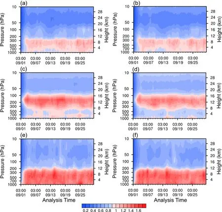
Fig.5.The RMS evolution of the difference between the two experiments HSCAT_EXP and CTRL for zonal wind analysis(a, c, e) and meridional wind analysis (b, d, f) in NH (a, b), TP (c, d), and SH (e, f).The X-axis is analysis time [coordinated universal time (UTC)], which is formatted as hour and minute above and month and date below.The following figures are in this time format.

Figure 7 is similar to Fig.5 but shows the geopotential height (Figs.7a, c, e) and temperature (Figs.7b, d, f).The difference between the geopotential height analyses between HSCAT_EXP and CTRL increases with the height for the northern hemisphere and tropics.In comparison, the assimilation of HSCAT-B OSW has a larger impact on the southern hemisphere, with the greatest impact below 850 hPa.The probable reason is that the conventional near-surface observational data in the southern hemisphere is very scarce, leading to a more profound impact of assimilating the near-surface satellite data in HSCAT_EXP.

Figures 7b, d, and f illustrate the temperature for the three regions, which shows that the maximum impact on the analysis is concentrated in the 700-1000 hPa layer, followed by the level near the tropopause (～100 hPa).The large influence on the model top layer is related to the framework of the GRAPES_GFS 4DVAR, which uses pressure as the control variable.Overall, the impact of data assimilation (DA)at the tropopause is larger in the tropics relative to the other regions.In contrast, the DA impact near the surface remains the largest in the southern hemisphere as it does for the wind and geopotential height.

In addition, Figs.5 and 7 show that at the beginning of the assimilation cycle (0300 UTC 1 September 2020), the influence of assimilating HSCAT-B OSW is relativelysmall.With the integration of assimilation effects, the impact of the assimilation extends to the whole troposphere after two days and reaches a balanced state.This result further demonstrates that the impact of assimilating the HSCAT-B OSW data is not only limited to the ABL, but also extends throughout the entire troposphere with a quick response after successive DA cycles.

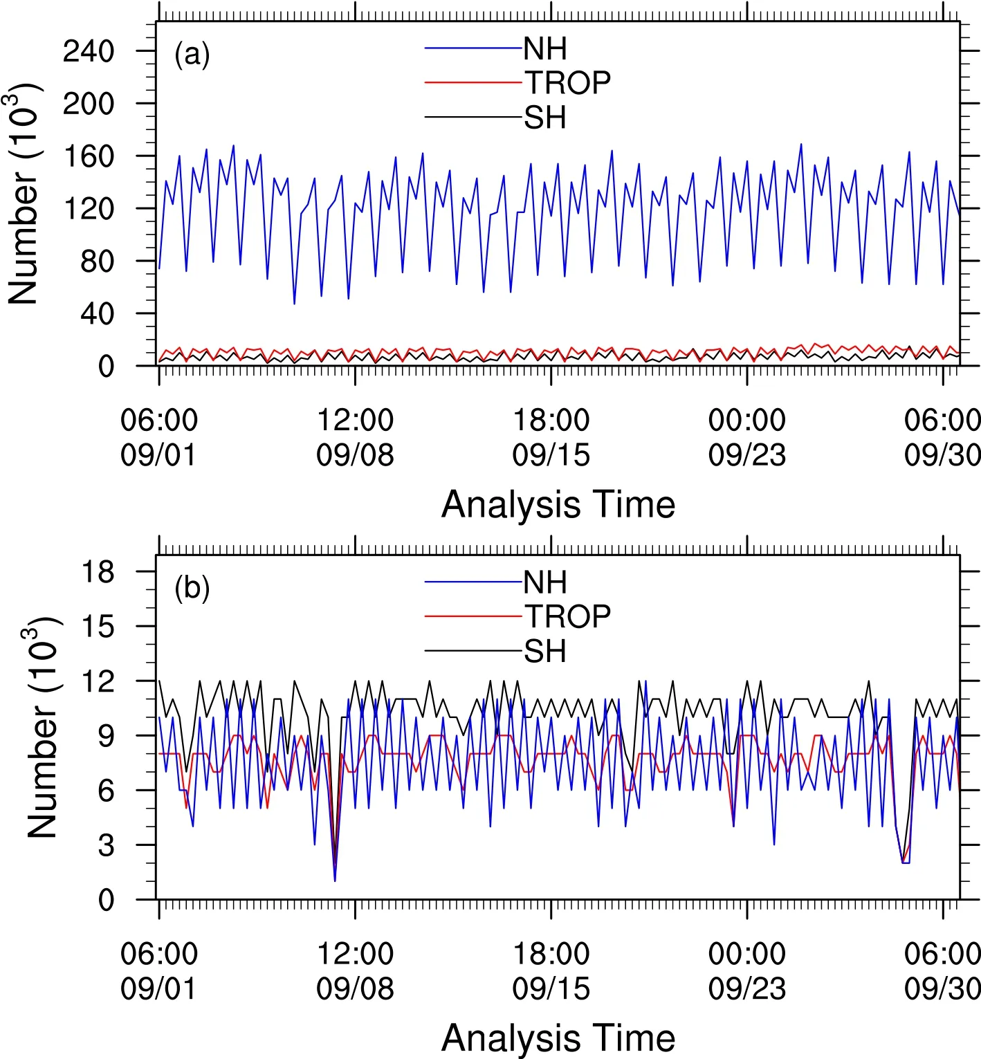
Fig.6.The number of assimilated wind vector observations (AIREP, TEMP, and AMVs) of the (a) CTRL experiment and (b) HSCAT-B OSW data of HSCAT_EXP experiment in the SH (black), TROP (red), and NH (blue).

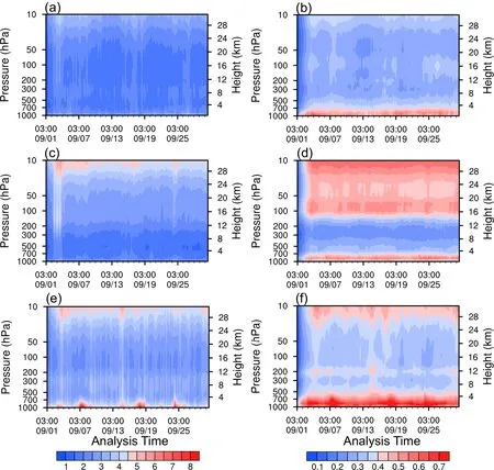
Fig.7.The same as Fig.5, but for the geopotential height (a, c, e, units: gpm) and temperature (b, d, f, units: K).

3.2.Impact on the GRAPES forecast

The RMSE and anomaly correlation coefficient (ACC)are two commonly used metrics in evaluating global medium-range numerical weather forecasts.We use these two metrics to assess the assimilation of the HSCAT-B OSW data on forecasts.

Figure 8 shows the RMSE difference in the wind forecasts between HACAT_EXP and CTRL in the northern and southern hemispheres and tropics.For the u-wind forecast in the northern hemisphere, the RMSE of HSCAT_EXP is reduced below 150 hPa during the first six days compared with the CRTL.In particular, the error reduction in the first 24 hours below 700 hPa passed the confidence interval test at the 95% confidence level.It is unclear why there is an increase in RMSE for the u-wind above 700 hPa within 0-72 hours and in the entire layer within 168-240 hours.For the v-wind forecast in the northern hemisphere, the RMSE differences are similar to the u-wind forecast, except that the RMSE below 150 hPa within 168-240 hours is lower in HSCAT_EXP.For the forecast of u- and v-wind in the tropical regions, the HSCAT_EXP experiment has a lower RMSE than CTRL below 70 hPa within 0-240 hours.In particular, the improvement of forecast skill at the midlower troposphere within 0-144 hours passed the confidenceinterval test at a 95% confidence level.For the forecast of uand v-wind components in the southern hemisphere, the RMSEs within 0-144 hours for almost the entire depth of atmosphere are reduced compared with the CRTL.Most especially, the RMSE reduction below 70 hPa within 0-96 hours has passed the confidence interval test at a 95% confidence level.

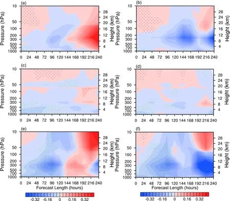
Fig.8.The RMSE difference (shaded) and its confidence interval test of the wind forecast between the HSCAT_EXP and the CTRL in (a, b) the northern hemisphere, (c, d) the tropical regions, and (e, f) the southern hemisphere (units: m s-1).The green (negative values) and red (positive values) dots have passed the confidence interval test at the 95% confidence level.The zonal wind, u, is indicated by panels (a), (c), and (e).The meridional wind, v, is indicated by panels (b), (d), and (f).

Figure 9 shows the forecast RMSE difference of the geopotential height and temperature between HSCAT_EXP and CTRL in the three regions.Compared with the CTRL,except for the levels above 30 hPa, the forecast RMSE of geopotential height is significantly reduced in HSCAT_EXP for all the three regions.Moreover, the regions with statistically significant differences at a 95% confidence level include the 250-50 hPa layer in the northern hemisphere and the 1000-50 hPa layer in tropical regions out to 168 hours, and the 1000-50 hPa layer in the southern hemisphere out to 96 hours.For the temperature forecast,the RMSE is reduced in HSCAT_EXP within 0-192 hours in all three regions, especially the southern hemisphere.The RMSE difference in 0-96 hour forecasts passes the confidence interval test at a 95% confidence level.The RMSE reduction of the temperature in the northern hemisphere and tropical regions is relatively small compared to the southern hemisphere.In addition, the RMSE reductions in the middle troposphere (400-200 hPa) in the tropical regions have passed the confidence interval test at a 95% confidence level.The comparison between Figs.9c-d indicates that the RMSE differences are different for geopotential height and temperature in the tropics, which may be related to the static instability caused by frequent convective activities and the low accuracy of cloud simulations in tropical regions.

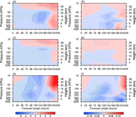
Fig.9.The same as Fig.8, but for the analysis field of (a, c, e) geopotential height (units: gpm) and (b, d, f) temperature (units: K).

Figures 10 and 11 show the ACC difference of the forecast fields of u, v, geopotential height, and temperature between the two experiments.They display qualitatively similar results compared to the RMSE analysis, except for a slight difference in the mid-lower tropospheric temperature forecast in the tropical regions.Moreover, for the RMSE and ACC, the forecast lead time and the vertical levels which have passed the confidence interval test at a 95% confidence level are nearly identical.

4.Summary

To reveal the influence of assimilating the HY-2B OSW observation on the analysis and forecast of the global numerical weather forecast model, this study designs an OSW data assimilation algorithm based on the GRAPES_GFS 4DVAR assimilation system, including data quality control, observational error estimation, and a data thinning scheme.The DA impact of the HY-2B OSW data is examined and analyzed by comparing the operational analyses and forecasts (i.e., the “CTRL” experiment) to those that additionally assimilate the HY-2B OSW (i.e., the“HSCAT_EXP” experiment).

The HY-2B OSW data is a high-accuracy observational product, resulting in a probability distribution of the OMB close to the Gaussian distribution, which means the data meets the requirements for variational data assimilation.Based on the GRAPES_GFS background field, the mean OMB of the u- and v-wind components of the HY-2B OSW are 0.038 and 0.034 m s-1, respectively, and the related standard deviations are 1.604 and 1.598 m s-1, respectively.

The GRAPES_GFS background field has obvious deviations from the HY-2B OSW observations.The horizontal distribution characteristics of the deviations are correlated with the features of major climate systems.There is an obvious westerly wind deviation in the westerlies, an easterly wind deviation in the tropical trade-wind zone, and a westerly wind deviation in the core areas of ENSO and the coastalareas of the main continents.Moreover, there is an obvious southerly wind deviation in the northern hemisphere and an obvious northerly wind deviation in the southern hemisphere.After assimilating the HY-2B OSW data, the deviations of the GRAPES_GFS OSW analysis fields are significantly reduced compared with the background field.

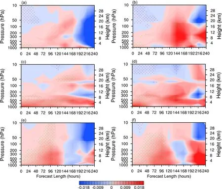
Fig.10.The ACC difference (shaded) and its confidence interval test of the wind vector forecast field between the HSCAT_EXP and the CTRL in (a, b) the northern hemisphere, (c, d) the tropical regions, and (e, f) the southern hemisphere.The green (negative values) and red (positive values) dots have passed the confidence interval test at a 95% confidence level.The zonal wind, u, is indicated by panels (a), (c), and (e).The meridional wind, v, is indicated by panels (b), (d), and (f).

The assimilation of HY-2B OSW data can influence the analysis of the whole troposphere instead of being limited to the ABL.After about two days of consecutive cycling assimilation, the HY-2B OSW information gradually extended to the whole troposphere, and then its influence on the analysis field remained relatively stable.It follows that the assimilation of HY-2B OSW data can significantly reduce the error of GRAPES_GFS wind analysis field in the mid-lower troposphere.By taking the ERA-5 reanalysis data as the reference, after assimilating HY-2B OSW data, the GRAPES_GFS analysis errors of the wind field in the mid-lower troposphere are significantly reduced by an average rate of about 5%.The reduction of the analysis error of near-surface wind is more significant, with an average reduction rate of about 10%.The GRAPES_GFS analysis errors of the temperature and geopotential height in the lower troposphere are also slightly reduced.As for the prediction, the assimilation of HY-2B OSW data can significantly reduce the tropospheric forecast errors of GRAPES_GFS in the southern hemisphere and tropical regions, greatly improving the forecast skill.

A key takeaway from the above results is that the assimilation of the OSW data not only greatly improves the analysis and forecast accuracy of the global numerical weather model in the ABL, but also significantly reduces the error of analysis and forecast of the whole troposphere in the southern hemisphere and tropical regions.However, there is stillroom for further improvement of the OSW assimilation effect, especially in optimizing the data thinning scheme.Data thinning is necessary due to the correlation of observational errors at adjacent grids and the mismatch between the horizontal resolutions of OSW observation and the model.In this study, the thinning scale of data is still empirically determined.Future studies will focus on improving the design of the optimal data thinning scheme to overcome the problems of data waste and insufficient information extraction in the current data thinning scheme and, ultimately, to improve the effect of OSW assimilation.

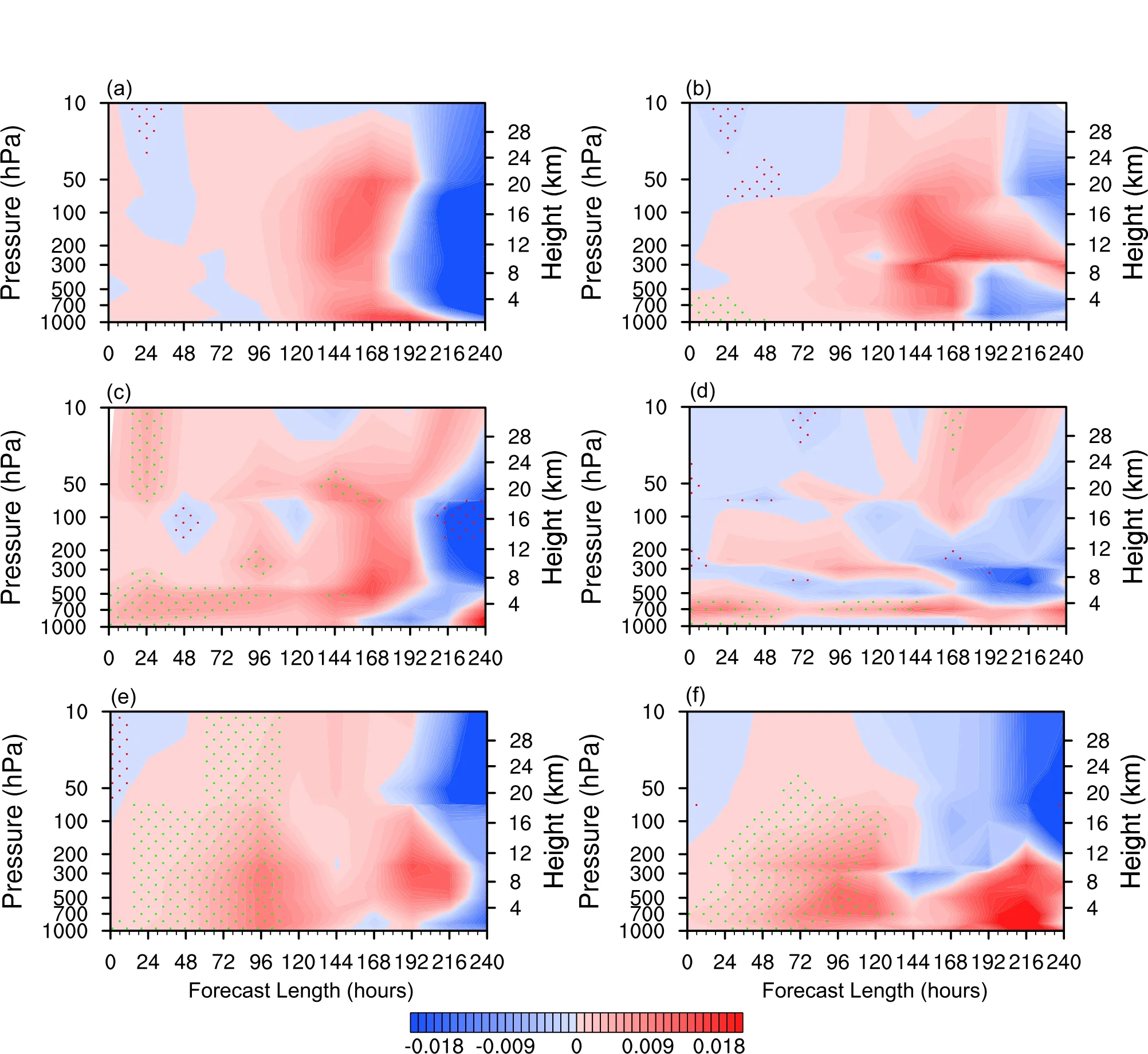
Fig.11.The same as Fig.10, but for (a, c, e) geopotential height field and (b, d, f) temperature field.

Acknowledgements.This research was supported by the Key Special Project for the Introduced Talents Team of Southern Marine Science and Engineering Guangdong Laboratory(Guangzhou) (Grant No.GML2019ZD0302) and the National Key R&D Program of China (Grant No.2018YFC1506205).