Distributed Radar Target Tracking with Low Communication Cost

Rui Zhang, Xinyu Zhang, Shenghua Zhou, Xiaojun Peng

Abstract: In distributed radar, most of existing radar networks operate in the tracking fusion mode which combines radar target tracks for a higher positioning accuracy. However, as the filtering covariance matrix indicating positioning accuracy often occupies many bits, the communication cost from local sensors to the fusion is not always sufficiently low for some wireless communication channels. This paper studies how to compress data for distributed tracking fusion algorithms. Based on the K-singular value decomposition (K-SVD) algorithm, a sparse coding algorithm is presented to sparsely represent the filtering covariance matrix. Then the least square quantization (LSQ) algorithm is used to quantize the data according to the statistical characteristics of the sparse coefficients. Quantized results are then coded with an arithmetic coding method which can further compress data. Numerical results indicate that this tracking data compression algorithm drops the communication bandwidth to 4% at the cost of a 16% root mean squared error (RMSE) loss.

Keywords: distributed radar; distributed tracking fusion; data compression; K-singular value decomposition(K-SVD) algorithm; sparse coding; least square quantization (LSQ)

1 Introduction

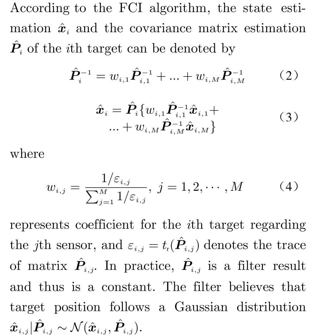
Distributed radar is a hot topic in the radar field and most of existing distributed radar systems operate in the track fusion mode, which can enhance radar target positioning performance through efficiently associating tracks from local sensors [1-5]. In contrast to local target tracks,the positioning accuracy after track fusion is much higher and target tracks are more smooth.Distributed track fusion algorithm can be classified into two types, namely centralized processing and decentralized processing. Most of early track fusion algorithms are decentralized track fusion algorithms, which combines target tracks from local sensors for a higher tracking performance. In [6], it is found that if a distributed tracking algorithm is designed under the assumption that observations from distributed radar sites are statistically independent, the covariance matrix will be under estimated. Therefore,mutual correlation of distributed observations should be considered and then Julier proposed the classical covariance intersection (CI) algorithm [7] that considers mutual correlation between local observations without needing to explicitly calculate it. However, the weights over local observations should be optimized, which typcially needs a high computation cost. In order to further reduce the computation cost, Niehsen proposed a fast covariance crossover (FCI) [8]algorithm to approximate the fusion weights by solving a linear optimization problem, so that the computational burden can be reduced, at the cost of a minor positioning performance loss. In centralized processing, point measures of a target from local radar sites are directly transmitted to a fusion center, in which a centralized track fusion algorithm is implemented. The later can reduce information loss, but it needs a high communication bandwidth and has a high requirement on the data processing capacity of the fusion center.

A reason to implement distributed track fusion algorithms lies in its low communication cost, compared with its signal-fusion counterpart.However, in real distributed radar systems, it is often found that the communication bandwidth requirement is not always low. For example, in a distributed sensor network, if each sensor transmits target tracks containing position and velocity information, the filtering result is composed of at least 42 numbers, namely, 6 elements to represent filtered target state and 36 elements to represent the filter covariance matrix. As the covariance matrix is symmetric in general, there are totally 27 numbers to transmit for each track. If 10 target tracks are updated during each coherent pulse interval (CPI) and each number is represented by 32 bits, there are 8 640 bits required.For a radar system with a 50 Hz data rate, the data rate for mere target tracks is about 422 Kbps. If a tracking algorithm such as particle filter[9, 10] is used, more bits will be required. In addition to other information, it is general easy to exceed 1-2 Mbps data rate in practice. This data rate is low for wired communications, but for wireless communications, it may be still high and thus should be further compressed [11, 12].

In this paper, we study how to compress distributed radar target track data. The distribution of the target state predictions is considered as a mixture distribution. The filtering covariance matrix is transformed to a vector and then the vector is considered as a multivariate random variable, whose covariance matrix is estimated through numerous numerical simulation.In [13], the singular value decomposition (SVD)is used to extract principle components of the covariance matrix. In [14], the principal component analysis (PCA) approach is used to compress the covariance matrices derived from realtime and sampling oscilloscope measurement. In[15], linear unbiased minimum variance (LUMV)is used to reduce the dimension of the matrix locus in the center of the minimized estimation error covariance, rather than the error covariance itself. However, the SVD based methods do not ensure the optimization results sparse. In practice, it is possible to optimize a dictionary matrix that can lead to sparse results, which will benefit the data compression performance [16]. In order to improve the sparsity of the covariance vector, we employ the dictionary learning method[17] and then optimize it to improve both the sparsity and matching performance. After solving a sparse constrained optimization problem,the coefficients are then quantized by the least square quantization (LSQ) algorithm [18]. The partitions are then encoded by an arithmetic coding method [19]. When the fusion center receives the compressed data, it first decompresses target track information and then employs the FCI algorithm for track fusion.

2 System Model

2.1 Signal Model

Consider a distributed radar system withMlocal radar stations connected to a fusion center through communication links. In the surveillance volume, there areNtargets in space and assume that these local radar sites can detect the targets.Assume that the target state at timetis denoted byxi,j ∈Cn×1, wherenstands for the dimension of the target state,idenotes the target, andjdenotes thejth sensor. Without loss of generality, we assume that the target state is composed of 3 target position components and 3 target velocity components. In this case,n=6.

If a local sensor detects the target, it will update the tracks regarding the targets. For most of existing tracking algorithms, a filtering result contains a filtered state denoted byxˆi,jand a covariance matrix, denoted byPˆi,j ∈Cn×nto describe the uncertainty of the target state. For simplicity, we assume that there is only one covariance matrix for each track update output.Assuming that each element occupiesmbits, the data rate of radar system isfr, the transmission data rate from distributed radar sites to the fusion center, denoted byC, can be written as

wherec1=n2mNMfrbit per second (bps)denotes the data rate for the covariance matrix,c0=nmNMfrbps denotes the data for the target state. Therefore, the covariance matrix occupies more data rate and in general, its structure is often highly featured. Subsequently, we focus on how to compressPˆi,jand to maintain the positioning performance.

2.2 Fast Covariance Intersection

2.3 Sparce-Coding and K-SVD

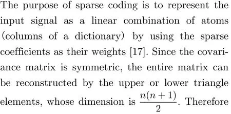
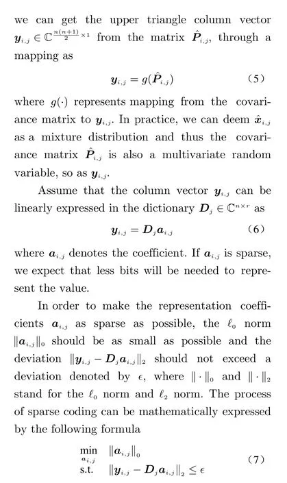
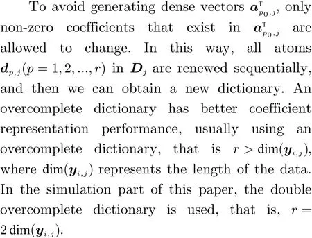
However,ℓ0norm in (7) is non-convex and its solution is an non-deterministic polynomial(NP) hard problem [20]. Thus, many approximate algorithms have been put forward to address this matter. Among them, the greedy algorithm is widely used for its simplicity and intuitionism. For example, matching pursuit(MP) [21] and orthogonal-matching-pursuit(OMP) [22] are two typical algorithms, and the later is used to solve the optimization problem(7).

In (7), the dictionaryDjis considered to be known. In fact, it is usually a fixed dictionary,such as the discrete cosine transform (DCT)matrix and discrete wavelet transform (DWT)matrix. In order to enhance the sparsity ofai,j,we can optimize it through data training. In dictionary learning, the K-SVD algorithm is widely used, which was first proposed by Aharon in [17].

In order to approximate statistical distribution of the covariance matrix for thejth radar site, we makeLnumerical simulations over different targets passing certain volume. Assume the filters will output covariance matrices, based on which the corresponding upper triangle column vectorsyj(i),i=1,2,··· ,Lare obtained. All the vectors are then combined to a matrix asYj=[yj(1),yj(2),...,yj(L)]. The K-SVD based dictionary learning method can be expressed by the following optimization problem

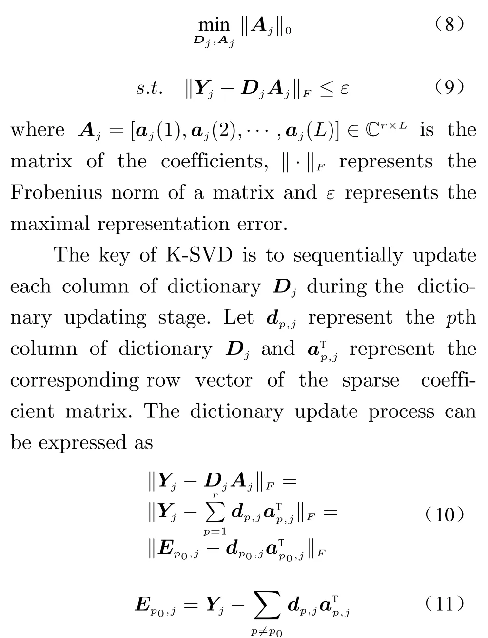
whereEp0,jis the residual matrix andp0means the updatingp0th column of the dictionary. The process of K-SVD algorithm of thejth radar is as follows

1) Initialization

AssumeDj(k)represents thekth iteration result of dictionaryDj. Initialize iteration numberk=0, and:

Step 1: initialize the dictionaryDj(0)∈Rn×rwith random elements orrrandomly selected covariance vectors.

Step 2: normalize the columns of dictionaryD(0).

2) Main Iteration

k=k+1, and:

Step 1: sparse coding

Use the orthogonal-matching-pursuit (OMP)[22] algorithm to solve the following formula

2.4 LSQ Quantization and Arithmetic Coding

After the sparse coding operation, the sparse coefficient vectoraioften has many coefficients close to zero. For the sparse coefficients, we can implement a quantization method that partitions the coefficients into different sections according to their probabilities. It has been proved that the LSQ method is optimal to quantize random variables with known statistical distributions and is thus be used as the quantization algorithm. The key now is to obtain the statistical distributions of the coefficients.

Ifarepresents the element of coeffificient,the probability density function of the coefficient is known asf(a), and the number of partitions is denoted byLq, LSQ can be used as the best nonuniform quantizer. The quantified reconstruction levelhkand decision boundarybkare

After the quantizaton operation, columnsai(i=1,2,··· ,N) of thejth radar are quantized to sequenceq(j). The greater the quantization bitsvis, the higher the matching performance and the higher the communication cost will be. For quantization sequenceq(j), entropy based encoding can be used to represent the results in less bits.

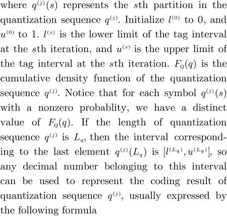
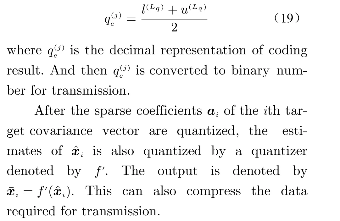
Arithmetic coding is a common entropy encoding, which can losslessly compress quantization sequence. The process of arithmetic coding can be expressed by

In order to reduce the communication bandwidth, this paper studies how to compress the covariance matrix, as shown in Fig. 1.

3 Compression Method

3.1 Dictionary Learning and Quantization Threshold Learning

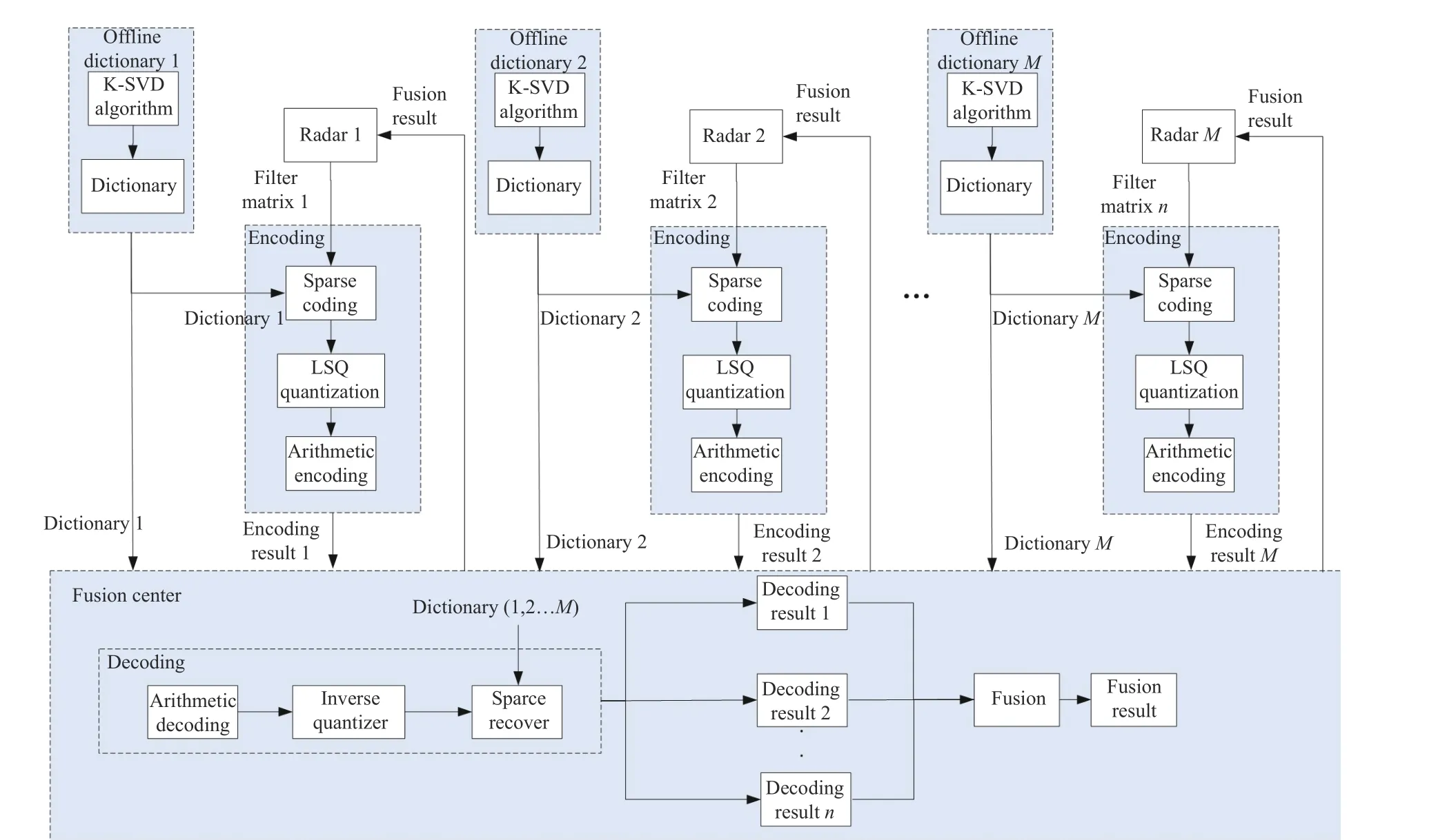
Fig. 1 Flow chart of the compression system

In general, for targets in space, the covariance matrix often follows a stable distribution, which depends on the SNR and tracking distance.Therefore, through numerical simulations, we can estimate the distribution ofyjand then obtain a data bank, based on which we can optimize for a dictionaryDjwith the K-SVD algorithm. The dictionary is obtained offline through numerical simulation or through numerous real data. Both local radar sites and the fusion center will store the dictionaryDj. Meanwhile, different radar sites may have different dictionaries, as a result of different radar operation parameters. It will be used later in the local radar sites to solve for sparse coefficients, and in the fusion center to recovery the covariance matrix for track fusion.

Given the dictionary matrix, one can also employ the sparse coding method such that the coefficientaican be calculated for all the tracking data. According to the coefficients, one can obtain the probability density function (PDF)estimates of different coefficients. Based on the PDF estimates, the quantization thresholds,denoted byb=[b1,··· ,bLq-1]Tcan be calculated according to the quantizerf. The thresholds will be stored in local radar sites. Given the thresholdsb, one can calculate the quantities for different partitions, denoted byh=[h1,··· ,hLq]T. The quantitieshwill be stored at the fusion center for recovery of the covariance matrix.

Meanwhile, in order to represent partitions,different partitions are encoded with the arithmetic coding method that maps all the partitions into a setQthrough a mapc. Assume thatqiis encoded tohq=c(qi) andx¯iis encoded tohx=c(x¯i).

3.2 Encoding at Local Radar Sites

The encoding operation is performed on local radar sites with the dictionaryDjobtained offline. ConsiderMdistributed radar sites andNtargets under track. For each target track, the following operations should be performed.

1) Step 1 Filtering and Mapping

According to the target track algorithm in use, update target track with an observation associated, yielding a target state estimatexˆiand a filter covariance matrixPˆi. According toPˆi, a vectoryiis obtained through the mappinggdefined in (5).

2) Step 2 Sparse Coding

Foryi, a sparse code method is used to obtain sparse coefficients and the results are denoted byai.

3) Step 3 LSQ Quantization

Elements ofaiis quantized by a quantizer denoted byq=f(a), which partitions the coefficient according to the thresholdsbcalculated offline. Then we can get quantization sequenceq(j). Meanwhile, the estimate of the target state can also be quantized through the quantizerf′with quantization thresholdsb′.

4) Step 4 Arithmetic Coding

Encode the sparse coefficients and the estimates of target tracks with the code mappingc.For all target tracks needing to update at the fusion center, the codes will be combined together and then will be transmitted through communciation links to a fusion center, together with auxiliary information.

3.3 Decoding at Fusion Center

1) Step 1 Arithmetic Decoding

A communication link at fusion center will output target tracks from different radar sites.For data from different communication links, different encoding rulesciwill be evoked to decode.

2) Step 2 State Estimates and Sparse Coefficients Recovery

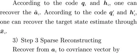
4) Step 4 Covariance Assembling

Using the properties of symmetric matrix,the column vectoryˆiis transformed into the covariance matrixPˆiby

whereg-1(·) means inverse transform ofg.

5) Step 5 Track Fusion

Now track data from all local radar sites are recovered and then track fusion algorithms can be implemented for a higher track performance.In track fusion, one should first correctly associate possible observations and then evoke the tracking algorithm in use. Of course, the track information can be feedback to local radar sites for a higher encoding performance in the next run, which will be studied in future.

4 Simulation Results

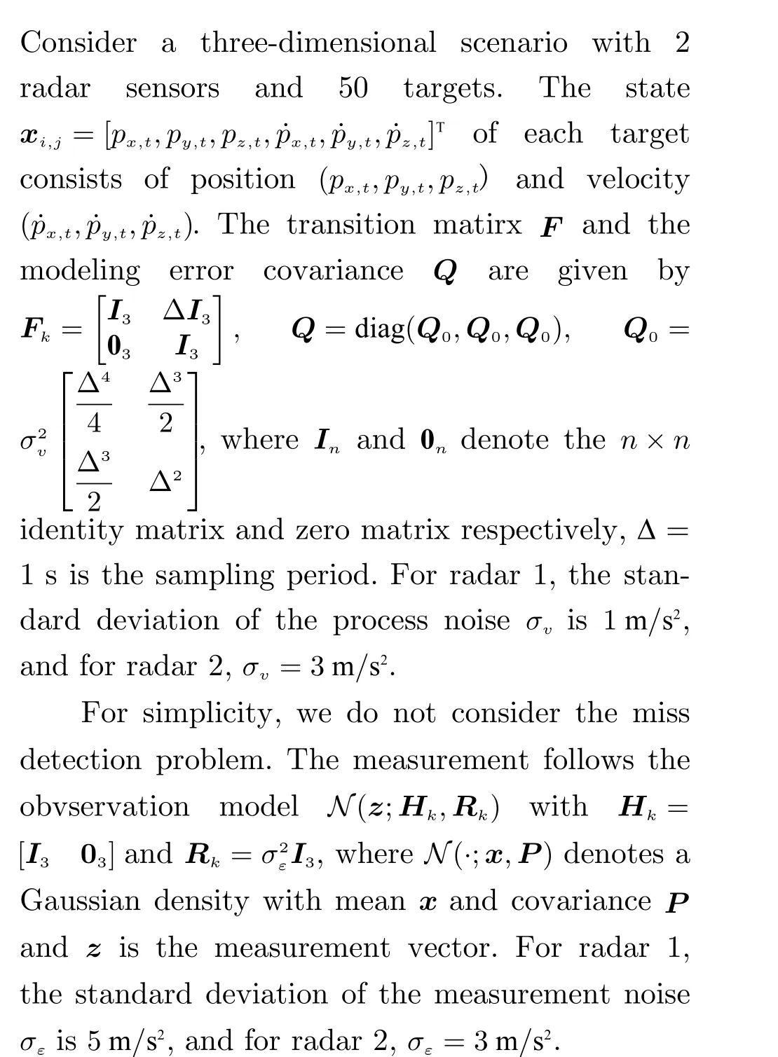
In dictionary learning, we setε=0.01 andL=3000. The number of columns in the overcomplete dictionary is twice the number of rows of input data. The deviation and maximum number of iterations are set the same as the sparse coding algorithm. We run 1000 Monte Carlo trials for each radar and use the root mean squared error (RMSE) to evaluate the distance error and F-norm to evaluate the difference between the compressed covariance matrix and the original covariance matrix.

Fig. 2 shows the elements ofaiafter K-SVD dictionary training and sparse coding. They-axis of the 50 targets signal represents the sparse coefficients after preprocessing, dictionary learning and sparse coding. Most of coefficients are close to zero after the sparsity operation.

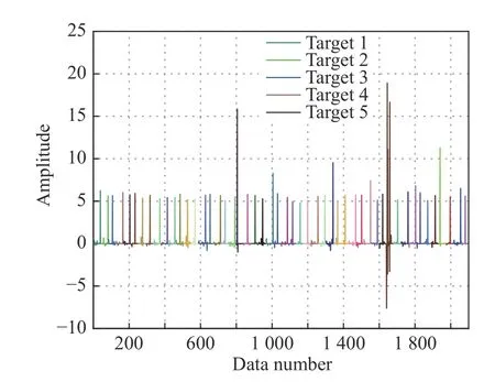
Fig. 2 The sparse coefficients of all targets after sparse coding at a given time, where different colors represent different targets

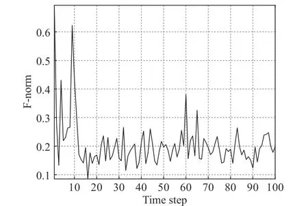
Fig. 3 The error F-norm of the original covariance matrix and compressed covariance matrix

Fig. 3 shows the error F-norm of the original covariance matrix and the covariance matrix transmitted to the fusion center after compression. Fig. 4 shows the RMSE of different methods, and Fig. 5 shows the compression ratio with time. These figures indicate that the compression method can efficiently compress the data in need for track fusion. However, the track performance will degrade slightly.

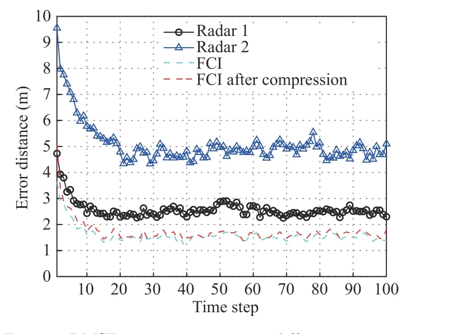
Fig. 4 RMSE error comparison in different scenarios

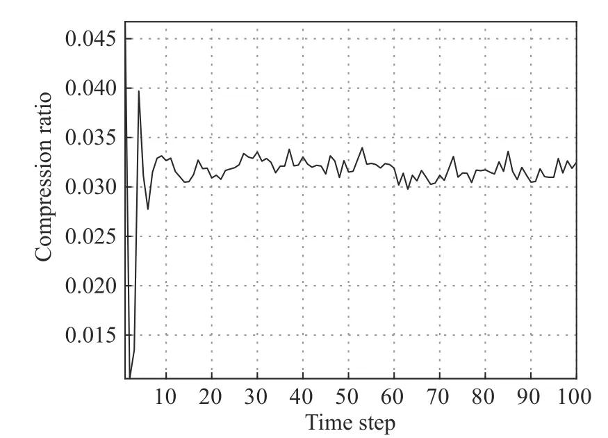
Fig. 5 The curve of compression ratio changes over time

5 Conclusion

In order to further reduce the communication bandwidth requirement for distributed track fusion, this paper studies the distributed radar track fusion algorithm with compressed local tracks. A dictionary learning and sparse coding method is introduced, which effectively reduces the data amount requirement for transmission.Through numerical results, it is found that the compression algorithm can efficiently suppress the data from local radar sites to the fusion center, but the track performance will degrade a bit.In our simulation configurations, we find that the compression ratio is 4%. Simultaneously, a 16%RMSE loss tracking performance will be induced.