Implementation of high-fidelity neutronics and thermal-hydraulic coupling calculations in HNET

Yan-Ling Zhu• Xing-Wu Chen • Chen Hao • Yi-Zhen Wang •Yun-Lin Xu

Abstract To perform nuclear reactor simulations in a more realistic manner, the coupling scheme between neutronics and thermal-hydraulics was implemented in the HNET program for both steady-state and transient conditions.For simplicity,efficiency,and robustness,the matrixfree Newton/Krylov (MFNK) method was applied to the steady-state coupling calculation. In addition, the optimal perturbation size was adopted to further improve the convergence behavior of the MFNK.For the transient coupling simulation, the operator splitting method with a staggered time mesh was utilized to balance the computational cost and accuracy. Finally, VERA Problem 6 with power and boron perturbation and the NEACRP transient benchmark were simulated for analysis. The numerical results show that the MFNK method can outperform Picard iteration in terms of both efficiency and robustness for a wide range of problems. Furthermore, the reasonable agreement between the simulation results and the reference results for the NEACRP transient benchmark verifies the capability of predicting the behavior of the nuclear reactor.

Keywords Coupling calculation · High-fidelity neutronics · Thermal-hydraulics · Matrix-free Newton/Krylov method · Transient simulation

1 Introduction

With the growing computing power and requirement of safety analysis [1], there has been interest in the highfidelity simulation of the nuclear reactor core [2-4]. The operational phenomena in the reactor to be simulated are very complex owing to the close interaction among various physical fields, particularly neutronics and thermal hydraulics[5,6].More specifically,the power density from the neutron flux significantly affects the thermal properties,which in turn has a powerful influence on neutronics through cross sections. Hence, to achieve a realistic prediction of reactor behavior under steady-state and transient conditions, the strong bond between neutronics and thermal-hydraulics must be considered.

Because the steady-state solution is generally regarded as the initial condition for transients[7],the first priority is to address the steady-state coupling of neutronics and thermal hydraulics. For steady-state coupling calculations,the Picard iteration has been studied and used extensively in high-fidelity simulation codes. However, convergence may be difficult and inefficient when the nonlinearity of the problem increases significantly [8]. Hence, some approaches have emerged to address the limitations of Picard iteration, such as relaxation, partially converging physics[8], and Anderson acceleration [9]. Alternatively, the fully implicit Jacobian-free Newton-Krylov (JFNK) method[10],with fast convergence and good robustness,has come into focus. However, most high-fidelity neutronics codes do not form the residuals required to implement JFNK.Therefore, the application of JFNK requires significant modifications to the algorithms of these well-developed codes. For simple implementation and good convergence performance, the MFNK method was proposed [11]. In contrast to the JFNK method, MFNK constructs residuals through the solutions of individual subsystems within the Picard iteration framework. Thus, MFNK can possess the advantage of implicit coupling while avoiding the reformulation of the coupled subsystems into a larger nonlinear system.

After the steady-state coupling calculation, the transient coupling simulation was emphasized.Although the implicit coupling scheme mentioned above has been applied to the nodal method for transient coupling calculation [12], most transient coupled systems still adopt the operator splitting(OS) method to compromise between computational burden and accuracy.Numerical instability may occur because of the explicit exchange of coupled information. Some improvements to the OS method have been developed,and the two main strategies are using staggered time mesh and higher-order time discretization of the nonlinear terms[12].

The high-fidelity Neutron Transport Program(HNET)is a 2D/1D transport code based on multilevel acceleration theory[13,14].The accuracy and efficiency of HNET have been verified against various steady-state and transient tests[15, 16], but only for problems without thermal-hydraulic feedback. To consider the interaction between neutronics and thermal hydraulics, a simplified internal thermal-hydraulic module was developed in HNET to provide thermal-hydraulic feedback. The MFNK method was adopted for the steady-state coupling calculation.Moreover,the OS method with a staggered time mesh was applied to the transient simulation.

The remainder of this paper is organized as follows. In Sect. 2, the MFNK method and the estimation of the associated optimal perturbation size are introduced. Section 3 describes the implementation of the coupling neutronics with thermal hydraulics. An assessment of the MFNK method for the VERA core physics benchmark problem 6[17] and the numerical results for the NEACRP transient benchmark [18] are presented in Sect. 4. Finally,conclusions are drawn in Sect. 5.

2 Matrix-free Newton/Krylov method

2.1 Derivation of MFNK method

The MFNK method is based on the block Gauss-Seidel(BGS)-style Picard iteration. For the nuclear reactor nonlinear system considering neutronics and thermal hydraulics, the BGS-style Picard iteration alternatively solving each physical field can be written as in Eqs. (1)and(2).

where vector x denotes the fuel temperature, coolant temperature, and coolant density in the thermal-hydraulic model, and y denotes the power density derived from the neutron fluxes.FTHand FNrepresent the thermal-hydraulic solver and neutronics solver, respectively. Superscript k represents the iteration number. Because the coupled problem is implicit, the overline in Eqs. (1) and (2) indicates that the corresponding variables should be transformed further. In this sense, FTHand FNshould be regarded as abstract solvers involving the total required operations, rather than only an actual solver. For brevity,the tilde is omitted from the expressions in the subsequent analysis.

When the coupled problem converges, the solutions to Eqs. (1) and (2) must be consistent, which implies that the nonlinear system can be expressed in terms of a residual form, as in Eq. (3).

where J(yk) represents the Jacobian matrix.

The linear system Eq.(5)can be solved using the Krylov subspace method, where the Jacobian matrix is only utilized for the action of the matrix-vector product. In this scheme, the Jacobian matrix-vector product can be approximated by the finite difference approximation to avoid assembling the Jacobian matrix explicitly, as shown in Eq. (6).

The MFNK iteration is repeated until the convergence criteria are met. Subsequently, thermal-hydraulic results are obtained based on the converged value y. From the above analysis, it can be found that only the solution and not the residual of individual subsystems are necessary to implement MFNK.

2.2 Optimal perturbation size

The finite difference approximation implemented in Eq.(6)results in truncation and rounding errors,as well as convenience. The truncation error is proportional to the perturbation size, whereas the rounding error is the opposite. Therefore, a balance should be found between the truncation error and the rounding error through the selection of the perturbation size.

Xu [11] proposed a method to estimate the optimal perturbation size.Assuming that y,v,and ε are given at the machine precision, the error edintroduced by the finite difference approximation can be arranged into Eq. (8).

where, skis the increment of the kth Newton iteration.

By replacing ‖F＇（y）‖and γ in Eq.(9)with that given in Eqs. (10) and (11), the optimal perturbation size is computed using Eq. (12).

3 Implementation of coupling neutronics

with thermal-hydraulics

3.1 High-fidelity neutron transport program(HNET)

HNET is a 3D whole-core transport code capable of performing high-fidelity neutron transport calculations for both steady-state and transient problems. The 2D/1D method with multilevel generalized equivalence theorybased CMFD acceleration (gCMFD) was developed in HNET for transport calculations. Specifically, the 2D method of characteristics(MOC)was utilized for the radial solver, and the two-node nodal expansion method is used for the axial dependency. The 2D and 1D solutions were coupled using transverse leakage. To decrease the computational cost of the CMFD,an innovative self-developed RSILU-preconditioned GMRES solver was utilized for the CMFD linear system. Regarding transient simulation, the multilevel predictor-corrector quasi-static scheme, together with the multilevel gCMFD acceleration, was developed to accelerate the time-dependent neutron transport calculation. Additionally, HNET employs the 47-group HELIOS library to provide cross sections, and the subgroup method was used for resonance self-shielding calculations. A detailed description of the transport calculations in HNET can be found in the References[14, 15, 19, 20].

3.2 Thermal-hydraulic model

To provide the fuel temperature, coolant temperature,and coolant density to the neutronics field, a simplified internal thermal-hydraulic module was developed in the HNET.For pressurized water reactors,the module consists of a 1D radial heat conduction model and a 1D axial heat convection model, which have been proven to be effective for a wide range of applications [8].

The heat-transfer calculation began with a cylindrical conduction equation. Because of the large ratio of axil length to radius and the axisymmetric geometry, axial and circumferential heat transfer can be ignored; thus, only radial heat conduction is considered for the fuel rods,as in Eq. (13).

where T, ρ, cp, k, and r denote temperature, density,specific heat, thermal conductivity, and radius, respectively. The volumetric power density q＇＇＇contributes to the fission reaction.

In addition, it is necessary to provide boundary conditions between heat conduction and convection. The heat flux transferred from the pellet to the fluid is determined by the following boundary condition as in Eq. (14).

where TMand Tfare the temperatures of the cladding outer wall and coolant, respectively, and hwis the convective heat-transfer coefficient,which is determined by the Dittus-Boelter correlation.

In terms of the flow field, a single-channel model with the following reasonable assumptions is applied: (a) Each assembly is defined as a channel region. In addition, no cross-flow between the adjacent channels was considered.(b) The coolant was always in the liquid phase. (c) The coolant pressure was approximately constant during the steady state and was fast transient.

Under these assumptions, the momentum conservation equation was removed.Thus,only the remaining mass and energy conservation equations were resolved in the flow field, and their general formulas in the axial direction are given by Eqs. (15) and (16).

3.3 Coupling implementation

The implementation of the MFNK method in the steadystate coupling calculation is shown in Fig. 1. Notably, two coupling configurations can be arranged according to the choice of the initial guess.Because the dimension of power density is small in comparison with thermal-hydraulic solutions, the power density was selected as the initial estimate in this study. Next, to initiate the MFNK scheme with an appropriate initial power density y, the Picard iteration was performed first.Specifically,according to a primary y, thermal-hydraulic solutions are calculated and then used to update the macroscopic cross sections.Then, based on the results of the transport calculation, a new yPicardwas obtained.

The MFNK method began after the initial guess calculation. Based on the given y, the Picard iteration was performed to form the residual, as described in Eq. (3).Subsequently, the Newton iteration was solved using the GMRES method,where the required matrix-vector product was approximated through a finite difference approximation with the optimal perturbation size. In each Newton step, a new solution y was updated. The iterative scheme was repeated until convergence was achieved. In addition, the maximum Krylov subspace dimension was chosen as two,and the transport solver was fully converged in each calculation.

In the transient simulation, the OS method was used to implement the transient coupling scheme. To improve stability, a staggered time mesh was applied to the OS method [21]. In this scheme, the two physical fields are

where ρ,v,and h denote the density,velocity,and enthalpy of coolant,respectively.z is the height in the axial direction and t represents time. LHand Acare the heated perimeter and the cross-sectional area of the channel, respectively.q＇＇w is the heat flux at the cladding surface, and q＇＇＇c is the heat source generated directly inside the coolant.

Fig. 1 Solution scheme of MFNK for steady-state coupling calculation

To solve the 1D radial heat conduction equations and 1D axial heat convection equations, the finite volume method is used to carry out spatial discretization, the theta method is adopted to discretize the time derivative terms, and the discrete formulas for the numerical calculation can be obtained.advanced for different time step sizes (Fig. 2). The thermal-hydraulics problem was solved first with one-half of the neutronics time step. Subsequently, based on the updated thermal-hydraulic conditions, the neutronics solver was invoked to calculate the neutron flux. Then, the thermal-hydraulics solver was advanced again using the new power density with one-half of the neutronics time step.

4 Numerical results and analysis

VERA Problem 6 [17] with different power levels and boron concentrations was first employed to study the convergence performance of the MFNK method. A comparison of the numerical results for MFNK, Picard, and Picard with relaxation is presented in this section. Subsequently, the NEACRP transient benchmark [18] was used to preliminarily test and verify the transient coupling calculation. The corresponding results were compared with reference solutions for verification.

4.1 Assessment of MFNK performance

VERA Problem 6 describes a single fuel assembly problem under typical full-power and nominal thermalhydraulic conditions, which are presented in Table 1. The assembly consisted of 264 fuel rods,24 guide tubes,and an instrument tube at the center. Meanwhile, there were six intermediate grids and two end grids in the assembly along the axial direction. More detailed geometric and material specifications are provided in [17].

For VERA Problem 6,the transport equation was solved using the 2D/1D method via gCMFD acceleration. Based on the 47-group HELIOS library, nuclide density, and temperature, the cross sections were obtained through resonance treatment. Figure 3 illustrates the discretization of MOC mesh in radial direction, the heterogeneous fuel pins are divided into 56 flat source regions (FSR), and the reflector cells use the 2 × 2 Cartesian sub-mesh. Inaddition, a ray spacing of 0.03 cm with 64 azimuthal angles and a Tabuchi-Yamamoto polar quadrature using 3 polar angles per half-space were utilized for MOC calculation. The active fuel region was divided into 49 axial layers, similar to VERA Problem 3 [17]. Furthermore, the core plates, nozzles, and grids were explicitly modeled for the transport domain. The radial boundaries were set to be reflective,and the vacuum boundary condition was applied axially, owing to the top and bottom water reflectors. For the thermal-hydraulic domain,each fuel pin,including the fuel pellet, gap, and cladding, was explicitly modeled and calculated individually using the radial power density inside the fuel pin. The discretization of the coolant channel in the axial direction is the same as that in the transport calculation. In addition, the inlet coolant conditions were adopted for the bottom structural material below the active fuel, whereas the average exit conditions of the coolant at the top of the active fuel region were used as the top structural material.

Fig. 2 (Color online) OS method with staggered time step

Table 1 Nominal thermal-hydraulics conditions

Fig.3 (Color online)The division of MOC mesh in radial direction:a fuel pin; b reflector cell

Generally, a fission source is used to measure the convergence of a coupled system.To evaluate the convergence behavior of MFNK,a strict convergence criterion using the power density residual norm was set for VERA Problem 6,as in Eq. (17).

where RMS is the root mean square of the residual vector and n is the linear system dimension.

First, according to Eq. (6), the influence of perturbation size on the MFNK method was investigated through VERA Problem 6.To test the behavior of the optimal perturbation size defined by Eq.(12), three empirical perturbation sizes were considered for the comparison.The first was a simple empirical perturbation with a constant value of 0.001. The second method is based on Pernice’s method [22].

where b is a constant whose magnitude is within a few orders of magnitude of the square root of the machine round-off.

Figure 4 illustrates how the perturbation size affects the convergence behavior of the MFNK method for VERA Problem 6. It can be observed that MFNK with a constant perturbation size converges very slowly.The performances of the other two empirical perturbation sizes are relatively consistent, and their residual norms seem to stagnate around 0.1. By contrast, MFNK with an optimal perturbation size can converge further and satisfy the convergence criterion. The primary reason is that the optimal perturbation size can reduce the error introduced by the finite difference approximation even when the residual norm becomes small, whereas the empirical ones cannot.Hence, the optimal perturbation size is used in the following analysis.

Subsequently,a convergence analysis was performed by comparing the results between the MFNK and Picard methods. Notably, in order to make an appropriate comparison between the MFNK and Picard methods, the convergence history was monitored by the iteration index of the MOC, which is a time-consuming procedure, rather than their individual outer iterations.

Fig. 4 The effect of perturbation size in the MFNK method

The convergence history of keffand the maximum fuel temperature for VERA problem 6 are shown in Figs. 5 and 6,respectively.The results indicate that MFNK achieved a stable state quickly, whereas Picard initially exhibited oscillatory behavior. For instance, the oscillation of keffin MFNK was a maximum of 1 pcm, whereas the maximum variation of keffin Picard is approximately 38 pcm. In addition, as illustrated in Figs. 5 and 6, the solutions resulting from MFNK and Picard match well.

To further evaluate the performance of MFNK, VERA Problem 6 with a modification of the power level and boron concentration was simulated. Traditionally, relaxation has been introduced to Picard for better convergence behavior.Hence, Picard and Picard with relaxation applied to the temperature solution were performed for comparison.Because the optimal choice of relaxation factor depends strongly on the problems, a relaxation factor of w = 0.5 was adopted in this paper [8]. The overall convergence performances of MFNK,Picard,and Picard with relaxation are summarized in Tables 2 and 3.In addition to the MOC iterations required for convergence, the total number of resonance calculations is also presented because of the relatively high computational cost. Notably, the resonance calculation was performed in the coupling scheme only when the maximum temperature change between two adjacent resonance calculations was larger than 1 K.

As shown in Table 2,MFNK and Picard with relaxation can considerably reduce the MOC iterations compared with Picard over all except for the 60% power level case.Although the three methods displayed a dependence on the power magnitude, MFNK and Picard with relaxation were less susceptible to the power level than Picard. Furthermore, it was observed that MFNK and Picard with relaxation could achieve convergence criteria in all cases,

Fig. 5 (Color online) Convergence history for keff

Fig. 6 (Color online) Convergence history for maximum fuel temperature

whereas Picard performed poorly and even diverged as the power level increased.This is primarily because increasing the power enhances coupling strength. However, Picard is generally unable to handle this stronger coupling. Additionally,the number of MOC iterations for MFNK was the same as or less than that for Picard with relaxation. More specifically, MFNK can decrease the number of MOC iterations from Picard with a maximum relaxation of 15.

In terms of boron perturbation, Table 3 demonstrates that varying the boron concentration does not affect the convergence behavior. As shown in Table 3, the performance of MFNK is slightly better than that of Picard with relaxation, and poor convergence can be found in the Picard results. Tables 2 and 3 show that the number of resonance calculations for MFNK and Picard with relaxation are comparable,and both are less than that for Picard as a whole.In other words,the cross sections can converge faster in MFNK and Picard with relaxation.

Figure 7 compares the power density residual norm of MFNK against Picard with and without relaxation with respect to the variation in the power level. In contrast to Picard with relaxation, the residual norm of MFNK dropped more rapidly in the 80% and 140% power cases. In addition, Picard converged at a markedly slower rate anddivergence behavior occurred in Picard at a 140% power level.

Table 3 Iterations to convergence for VERA Problem 6 at various boron concentrations

Based on the above analysis, it can be concluded that although MFNK does not perform as efficiently as Picard at the 60%power level,it can display a better convergence performance than Picard for a wider range of problems.Moreover, although the performance of MFNK is better than that of Picard with a relaxation factor of 0.5 in given cases,the opposite results may occur if the optimum values of the relaxation factor are selected.Nevertheless,it should be easier to improve the convergence rate and enhance the numerical stability when utilizing MFNK than when applying a relaxation scheme, because the optimal relaxation factor is problem-dependent and generally chosen empirically [21].

4.2 Transient simulation of control rod ejection

The NEACRP benchmark is a 3D PWR core transient problem constructed to simulate the ejection of a control assembly(CA)from the core under operational conditions.The assembly arrangement is shown in Fig. 8. Moreover,2-group macroscopic cross sections were set for 11 homogenized compositions. However, the NEACRP benchmark was originally specified for diffusion-based codes, resulting in a lack of total and self-scattering cross sections. To obtain an equivalent transport version, thetotal cross sections can be approximated to transport cross sections, and then the self-scattering cross sections are calculated using Eq. (20).

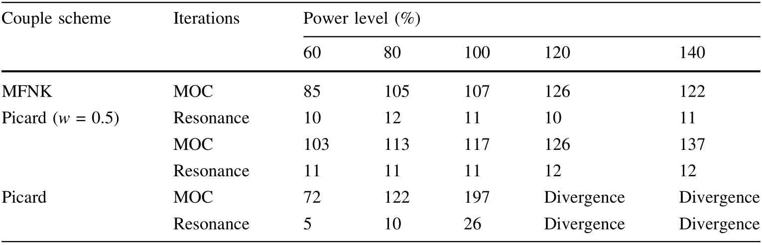
Table 2 Iterations to convergence for VERA Problem 6 at various power levels

Fig. 7 (Color online) Convergence behavior of the residual norm for VERA Problem 6 with power perturbation: a 80% power level; b 140%power level

Fig.8 (Color online)Radial layout of the quadrant core in NEACRP benchmark

where Σt, Σa, and Σsare the total, absorption, and scattering cross sections, respectively.

The NEACRP benchmark comprises six cases with different combinations of control arrangements, original positions, and power levels. A detailed description of the geometry, macroscopic cross sections, and initial configuration of the control assemblies can be found in[18]. In this study, cases A2 and B2 were considered to verify the accuracy of the transient simulation. Both cases were initiated by the rapid ejection of the CA in 0.1 s at hot full-power state;the CA to be ejected is marked by a circle in Fig. 8. Specifically, the symbols A and B represent the ejected CA of cases A2 and B2, respectively.

To resolve the NEACRP benchmark using the transient 2D/1D transport solver in HNET [15], the geometry was uniformly discretized into an FSR mesh size of 0.7202 cm × 0.7202 cm for the MOC calculation. Additionally,the ray spacing for the NEACRP benchmark is the same as that for VERA Problem 6.From bottom to top,the active zone was divided into 26 layers with heights of 7.7,11, 15 (21 layers), 12.8 (2 layers), and 8.0 cm, which differed from the division of the NEACRP benchmark for high accuracy of results.A reflective boundary was used to the west and north because of symmetry, whereas the rest used vacuum boundary conditions. Concerning the thermal-hydraulic calculation, an average fuel pin, representing all fuel pins of the associated assembly,was modeled in detail to obtain the radial temperature distribution by applying the average assembly power density. In the axial direction, the separation of the coolant channel was consistent with that of the transport calculation.

The steady-state thermal-hydraulic conditions are listed in Table 4. The relation between thermal properties, such as thermal conductivity and specific heat capacity, and temperature is derived from[18].Moreover,to consider the feedback effects from thermal hydraulics and boron concentration, the macroscopic cross sections for each composition are defined by Eq. (21).

Table 4 Steady-state thermal-hydraulic characteristics

where ρ, Tm, Tf, and C are the moderator temperature,moderator density, fuel temperature, and boron density,respectively. The subscript 0 represents the reference values.

A comparison of steady-state and transient solutions for cases A2 and B2 is given in Table 5.The reference results listed in Table 5 were derived from [23]. As shown in Table 5, there is good agreement between the simulation and reference results. The critical boron concentration at the steady state deviated slightly from the reference value,and the maximum difference was approximately 31 ppm,which is considered acceptable. In addition, the representative parameters in the transient process coincided well with the reference.

Figure 9 depicts the evolution of the core-normalized power and reactivity for case A2. Here, the adopted reference solutions are computed using the PARCS code[24].As indicated, the HNET results for case A2 are in agreement with that of PARCS. The slight deviation in the normalized power and reactivity curves can be explained by the difference in the neutronics methodology. The NEACRP benchmark is resolved by neutron transport calculations in HNET,whereas the nodal method is used in PARCS. In addition, as illustrated in Fig. 10a, there is no significant difference in the responses of the coolant exit temperature to the CA ejection between these two codes.Because the result of the Doppler temperature from the PARCS is not provided in [24], Fig. 10b plots only the solution of the HNET. From Fig. 10b, an increase in the average Doppler temperature owing to power increments is observed, which behaves as expected.

As shown in Figs. 11 and 12, to further test the level of agreement,a closer analysis of the axial relative power and radial normalized power for case A2 was performed at 0 s,0.1 s, and 5 s. The relative error e is defined by Eq. (22).

where calc represents the values calculated by HNET, and ref is the reference value derived from PARCS [24].

The normalized power in the pin and assembly levels are calculated using Eqs. (23) and (24).

where Ppinand Passemdenote the axial-integrated power per fuel pin and per fuel assembly, respectively; Npinand Nassemrepresent the total number of fuel pins and fuel assemblies, respectively; and Pcoreis the core power.

With respect to the axial relative power, no significant difference between HNET and PARCS is observed in Fig. 11.Figure 12 shows that the results of assembly level normalized power at the considered temporal points from HNET agree well with PARCS. Moreover, because the NEACRP benchmark was performed using a transient transport solver, the pin-wise power distribution can be obtained directly without power reconstruction. Figure 13 depicts the pin-wise radial normalized power for case A2 at 0.0 s and 0.1 s. The comparison shows that the pin power in the center increases significantly after the withdrawal of the control rod, which coincides with the sharp increase in power observed in Fig. 9.The above results prove that the evolution of the power distribution can be effectively captured when the reactivity is being inserted.

Table 5 Steady-state and transient calculation results

Fig. 9 (Color online) Transient responses in case A2: a normalized power; b reactivity

Fig. 10 (Color online) Transient responses in case A2: a coolant exit temperature; b core averaged Doppler temperature

Fig. 11 (Color online) Axial relative power for case A2: a time at 0.0 s; b time at 0.1 s; c time at 5.0 s

Fig.12 (Color online)Relative error of assembly normalized power for case A2 in quarter core geometry(%):a time at 0.0 s;b time at 0.1 s;c time at 5.0 s

Fig. 13 (Color online) Pin normalized power distribution for case A2 in quarter core geometry: a time at 0.0 s;b time at 0.1 s

Finally, because the thermal-hydraulics feedback is provided at the assembly level for the NEACRP benchmark, Fig. 14 shows the local temperatures in assemblies C-3 and B-8, where the highest and lowest powers appear,respectively. It can be observed that there are obvious discrepancies for fuel centerline temperatures between the two assemblies. As shown in Fig. 14b, the increase in temperatures between 0 and 5 s in assembly B-8 is larger than that in assembly C-3, particularly the fuel centerline temperature.

5 Conclusion

The primary objective of this study was to couple neutronics with thermal hydraulics in HNET. First, a simplified internal thermal-hydraulic module was developed for thermal properties. Subsequently, a steady-state coupling calculation is achieved by implementing the MFNK method. Next, the OS method with a staggered time mesh was used to accomplish the transient coupling simulation.

The investigation of the perturbation size shows that the optimal perturbation size can significantly enhance the convergence of the MFNK method compared with the empirical perturbation size.With respect to VERA problem 6 at different power levels and boron concentrations, the MFNK method is slightly sensitive to the feedback intensity and can considerably reduce the computational cost compared with the Picard iteration in most cases.It can be proven that the MFNK method is more stable and efficient than the Picard iteration for a wider range of problems.Notably,the performance of MFNK is as good as or better than that of Picard with relaxation, and there is no requirement for input data in MFNK compared with the relaxation approach.Furthermore,the numerical results for the NEACRP transient benchmark are in agreement with the reference values, indicating the validation of the transient coupling calculation in the hot full-power state. In conclusion, the results demonstrate that the neutronics and thermal-hydraulics coupling simulation is effectively performed in HNET under both steady-state and transient conditions.Author contributions All authors contributed to the study conception and design. Material preparation, data collection and analysis were performed by Yan-Ling Zhu, Xing-Wu Chen, Chen Hao, Yi-Zhen Wang, and Yun-Lin Xu. The first draft of the manuscript was written by Yan-Ling Zhu, Chen Hao, and Yi-Zhen Wang, and all authors commented on previous versions of the manuscript. All authors read and approved the final manuscript.

Fig. 14 (Color online) Local temperatures and change in temperatures in the assemblies with the highest and lowest powers: a local temperatures; b change in temperatures between 0 and 5 s