EXTREMA OF A GAUSSIAN RANDOM FIELD:BERMAN’S SOJOURN TIME METHOD*

Liwen CHEN (陈丽雯) Xiaofan PENG (彭小帆)

School of Mathematical Sciences,University of Electronic Science and Technology of China,Chengdu 611731,China

E-mail: CherWenwen@163.com;xfpengnk@126.com

Abstract In this paper we devote ourselves to extending Berman’s sojourn time method,which is thoroughly described in [1–3],to investigate the tail asymptotics of the extrema of a Gaussian random field over [0,T]d with T ∈(0,∞).

Key words tail asymptotics;sojourn time;Gaussian random field;extreme;stationarity

1 Introduction

In 1967,Pickands [4] first deduced the asymptotics of the extrema of a zero-mean stationary Gaussian process,which opened the door for research on the extremum distribution of Gaussian process.Two years later,Pickands [5,6] used a rather complex but very effective method to find the asymptotics of Pasu→∞,and came up with a finite and nonnegative constant,named Pickands constant by later researchers.Pickands’ method has had a profound effect on this research area.However,Pickands’ original proof used the upcrossing probabilities and thus looked a little complicated.Later,Piterbarg [7–11] introduced the double sum method;this verified Pickands’ results and was used extensively in [12–20].These works have greatly enriched the exploration of Gaussian extremum.Pickands’ and Piterbarg’s methods both proposed the Pickands constant

which was related to the asymptotics of Gaussian process.Here,Bαis a standard fractional Brownian motion with Hurst indexα/2,α∈(0,2].Another method,which we call the sojourn time method,was introduced independently by Simeon M.Berman [1–3],who also made an important contribution to the study of the extrema of random processes.Compared with the double sum method,this approach presents a new represention of Pickands constant;we call it the Berman constant:

Let {X(t),t ∈[0,T]d} be a centered stationary Gaussian random field with continuous trajectories,unit variance and correlation functionr(t)=r(|t|),|t|=(|t1|,|t2|,···,|td|),satisfying

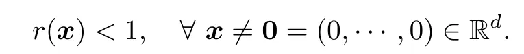
Throughout this article,we use bold letters to denote vectors in Rd.All operations between the vectors are meant to be componentwise.For example,for any given s=(s1,···,sd) ∈Rdand t=(t1,···,td) ∈Rd,we write s/t=(s1/t1,···,sd/td),and write ts if at least one element in t is strictly larger than the corresponding element in s.Inspired by Pickands [4],we assume that there exist v(u)=(v1(u),···,vd(u)) with limu→∞min1≤i≤dvi(u)=∞and some continuous functionsh(t),t ∈Rdwithh(0)=0 andh(t)＞0,∀t≠0 such that

holds for any compact set K ⊂Rd.Then,by (A.1.5) in [29],we know that 1 -r(t) is of regular variation inddimensions.

The main idea of our proof to investigate the tail asymptotics of the extremum of a stationary Gaussian random field is consistent with that of Berman [3].However,we make some changes and simplify the proof procedure to a certain extent.Berman assumed that,for a stationary Gaussian process with correlation functionr(s),1 -r(s) is of regular variation.In this article,we give a sufficient condition (1.1) for regular variation.Moreover,instead of using Fernique inequality (see,e.g.,Theorem 2.1.1 in [30]) and the weak convergence criterion employed by Berman,we use the Sudakov-Fernique inequality (see,e.g.,Theorem 2.9 in [31])and Borell-TIS inequality (see,e.g.,Theorem 2.1.1 in [32]),and apply the conclusions of [33,Problem 4.11] to prove the weak convergence of a Gaussian random field,all of which effectively simplifies the proof.

The rest of the paper is organised as follows: in Section 2,we present the main conclusions of the paper,and the corresponding proofs are displayed in Section 3.The related lemma used in the proof is given in the Appendix.

2 Main Result

For notational simplicity we set

wherevi(u) is related to the condition (1.1).Define the sojourn time on [0,T]das

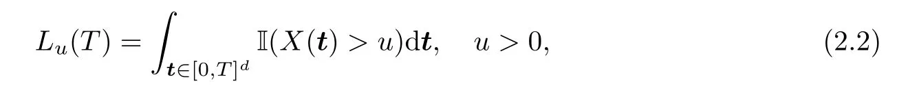
of which I(·) is an indicator function.We define the corresponding Berman constant as

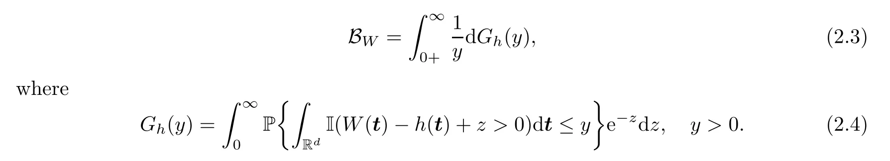
Here {W(t),t ∈Rd} is a Gaussian random field with stationary increments and continuous trajectories,and satisfies

withhgiven as in (1.1).(Note: Not all functionshsatisfying (2.5) can define a Gaussian random field as above.However,this is guaranteed ifhappears as the limit in (1.1),since then,by Kolmogorov’s Compatibility Theorem (see,e.g.,Theorem 5.4.8 in [34]),we can find out the corresponding random field.)

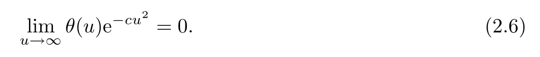
Theorem 2.1Let {X(t),t ∈[0,T]d} be a centered,sample path continuous,stationary Gaussian random field with unit variance and correlation functionrsatisfying (1.1) for some functionshand v.Letθ(u),LuandGhbe given in (2.1),(2.2) and (2.4),respectively.Denote byFuthe distribution function ofθ(u)Lu(T).Assume that,for anyc ＞0,

If,for arbitrarily largeλand1=(1,···,1) ∈Rd,there exists some (α1,α2,···,αd)＞0and a sufficiently smallδ ＞0 such that

holds for any positive continuity point ofGh(·).

Theorem 2.2Furthermore,under the assumptions of Theorem 2.1,if there exist some positiveCandγsuch that,for sufficiently largeu,

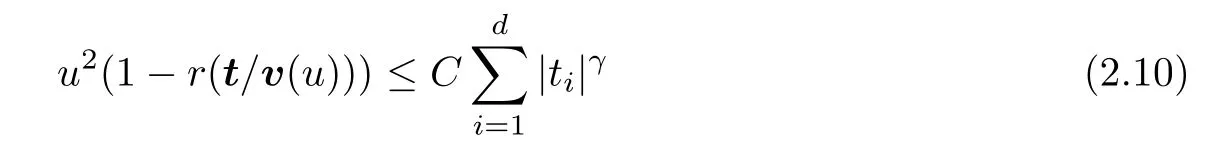
holds uniformly for t on any compact set K in Rd,then we have

where the Berman constant BWis defined as in (2.3).

Example 2.3Let {X(t),t ∈[0,T]d} be a centered stationary Gaussian random field with correlationr(t) satisfying (2.8) and,t →0for some (α1,···,αn)＞0.Then,we havevi(u)=u2/αi,i=1,···,dand,fulfilling (1.1).Furthermore,by (2.5),,whereBαi(t),i=1,···,dare independent fractional Brownian motions with Hurst indexαi/2,respectively.It is straightforward to check that assumptions(2.6) and (2.7) in Theorem 2.1,and (2.10) in Theorem 2.2,are all fulfilled.

3 Proof of Main Result

Before continuing with the proofs,we explain some notation.For simplicity,we often write v instead of v(u).For anyλ∈R,we writeλ/v=(λ/v1(u),···,λ/vd(u)).Denote by Ψ(u)and byφ(u) the tail distribution function and the probability density function,respectively,of a standard normal random variable.It is well known thatφ(u)～Ψ(u)uasu→∞.

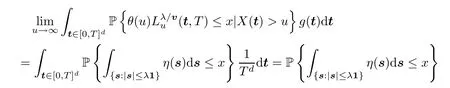
Proof of Theorem 2.1First,according to Fubini’s Theorem,we know that

By the stationarity ofX,we know thatg(t) is in fact the density function of uniform distribution on [0,T]d.Next,we present a conclusion of conditional convergence.For any t ∈(0,T)dand si∈Rd,i=1,···,m,

where,in the second equality,we have used a change of variable byy=u+z/uand the fact that{X(t+si/v)-r(si/v)X(t),i=1,···,m} are independent ofX(t).The last equality follows by the Dominated Convergence Theorem.

For each t ∈(0,T)d,{u(X(t+s/v) -r(s/v)X(t)),s ∈Rd} is a centered Gaussian field with the covariance function

which,by (1.1),converges toh(si)+h(sj)-h(si-sj).Furthermore,for eachz∈R+,

Thus,by the Inverse Limit Theorem,we get that

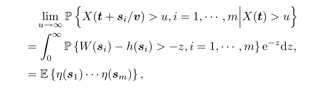
whereη(s)=I {W(s) -h(s)+Z＞0},s ∈Rdis a random field with values of 0 or 1,while Z is a unit exponential variable independent ofW.

For any vector λ＞0 and t ∈[0,T]d,set

which represents the sojourn time ofX(t) from a cube centered at t,with side lengths of 2λ.Then,for any fixed positive integersλandk,

holds for anyx∈(0,∞)Dλ,whereDλis the set of discontinuity points of the right-hand side function with Lebesgue measure 0.Consequently,by the Dominated Convergence Theorem,we get that

holds for anyx∈(0,∞)Dλ,which,together with Lemma 4.1 in the Appendix,implies that

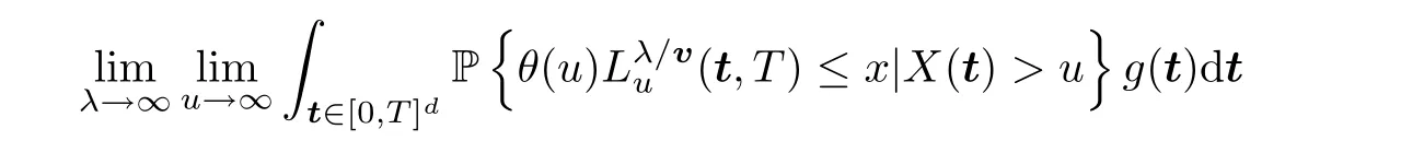
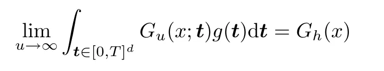
Multiplying on both sides of the above inequality byg(t),integrating over [0,T]d,and then passing to the limit,we get that

If the limit in (3.3) is equal to 0,then lettingε→0,we obtain that

holds for anyx∈(0,∞)S1,whereS1denotes the set of discontinuity points of left hand side of (3.4).Denoting byS2the set of discontinuity points ofGh(x),and combining (3.1),(3.2)and (3.4),we have that

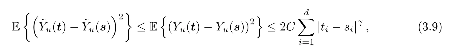
Last,to fill the gap of the proof,we need to show that the limit in (3.3) is actually 0.By(2.5.4) in [3],we know,for any s,t ∈[0,T]d,that

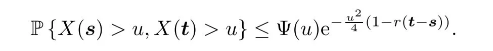
Thus,for arbitrarily smallδ∈(0,T),

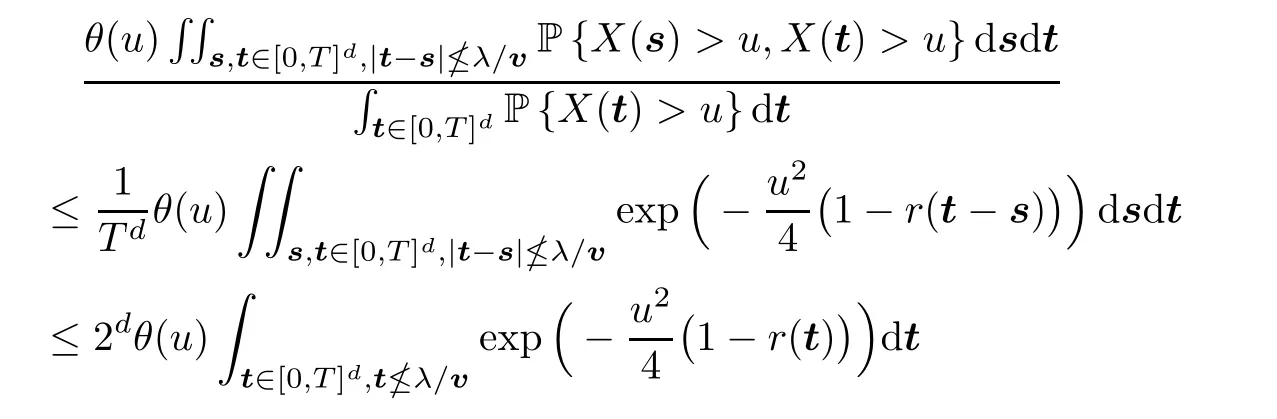
We know from (2.7) that,for sufficiently largeu,there exists some positive constantAsuch that

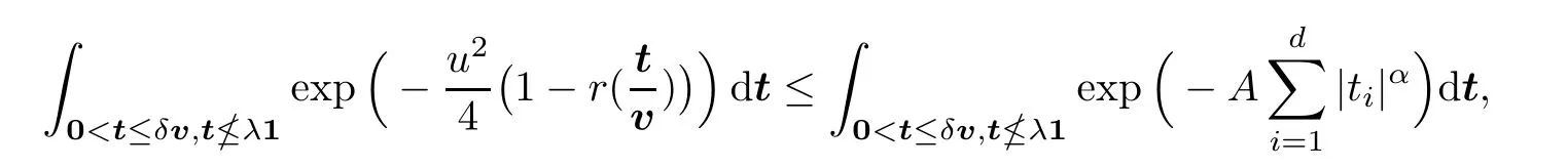
which tends to 0 asu→∞,and thenλ→∞.Furthermore,by (2.6) and (2.8),we have that

asu→∞.This completes the proof. □

Proof of Theorem 2.2According to Theorem 10.4.1 in [3],we know that

Therefore,it suffices to show that (3.5) is finite and that (3.6) is equal to 0.By Lemma 5.1 in[36],for anyS ＞0,we have that

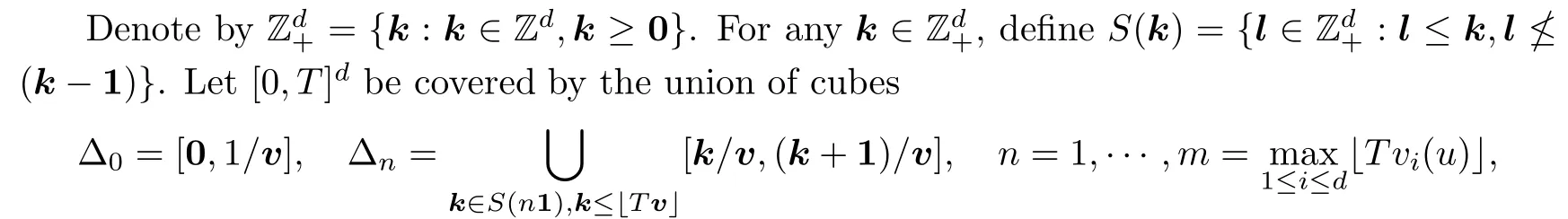
Decompose the cube [0,T]dinto small ones with side lengths of 1/v.Then,by the stationarity of random fieldX,

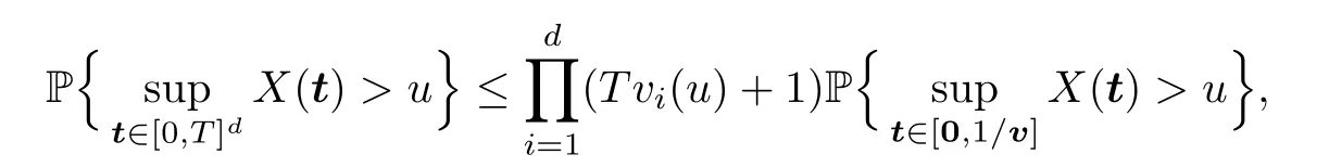
which,together with (3.7),implies that

In the remaining part of the proof,we show that the limit (3.6) is actually 0.

Then,for arbitraryε ＞0,by the stationarity ofX,we have that

and thus we only need to show that

For notational simplicity,define

By (2.10),we have,for any s,t ∈[0,T]dand sufficiently largeu,

and thus,by the Sudakov-Fernique inequality (see,e.g.,Theorem 2.9 in [31]),

Denoting byC1the above limit,for anyM ＞C1we have that

By the Borell-TIS inequality (see,e.g.,Theorem 2.1.1 in [32]),for large enoughu,

Next,since E {X(t)|X(0)=y}=r(t)y≤yholds for anyy≥0,we have

where the last inequality follows by the Borell-TIS inequality.Changing the variable byz=(u-y)/q(u) yields that

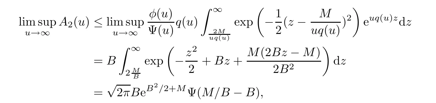
For the last termA3(u),note that

By a change of variabley=u-z/u,we get that

By (1.1) and (2.5),we know,for any s,t ∈[0,1]d,that

Hence,the finite-dimensional distributions ofconverge to that of {W(t),t ∈[0,1]d}.LetC([0,1]d) denote the Banach space of all continuous functions on [0,1]dequipped with sup-norm.By (3.9) and [33,Problem 4.11],the measures onC([0,1]d) induced byare tight for large u.Therefore,converges weakly asu→∞to {W(t),t ∈[0,1]d}.Furthermore,for eachz∈[0,2M],

Thus,the probability measures onC([0,1]d) induced byr(t/v)),t ∈[0,1]d} converge weakly,asu→∞,to that induced by {W(t) -h(t),t ∈[0,1]d}.Then,by the Continuous Mapping Theorem,we have that

Substituting (3.14) and (3.15) into (3.13),yield that

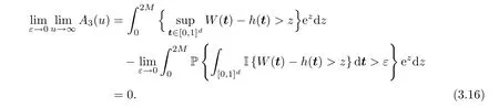
Finally,combining (3.11)–(3.12) with (3.16),and recalling (3.10),we get that

which verifies (3.8).This completes the proof. □

AcknowledgementsWe would like to thank Professor Enkelejd Hashorva and Professor Krzysztof D¸ebicki for many valuable discussions on the subject.

4 Appendix

Lemma 4.1IfXn,n≥1 is a sequence of increasing random variables which converges toXalmost surely asn→∞,then the corresponding distribution function ofXnconverges pointwise to that ofXasn→∞.

ProofFor anyε ＞0 andx∈R,we have that

The last term is 0,due to the almost sure convergence.Next,lettingε→0,and using the right continuity of the distribution function,establishes the proof. □