LSTM-Based Adaptive Modulation and Coding for Satellite-to-Ground Communications

Shiqi Zhang, Guoxin Yu, Shanping Yu, Yanjun Zhang, Yu Zhang

Abstract: Satellite communication develops rapidly due to its global coverage and is unrestricted to the ground environment. However, compared with the traditional ground TCP/IP network, a satellite-to-ground link has a more extensive round trip time (RTT) and a higher packet loss rate,which takes more time in error recovery and wastes precious channel resources. Forward error correction (FEC) is a coding method that can alleviate bit error and packet loss, but how to achieve high throughput in the dynamic network environment is still a significant challenge. Inspired by the deep learning technique, this paper proposes a signal-to-noise ratio (SNR) based adaptive coding modulation method. This method can maximize channel utilization while ensuring communication quality and is suitable for satellite-to-ground communication scenarios where the channel state changes rapidly. We predict the SNR using the long short-term memory (LSTM) network that considers the past channel status and real-time global weather. Finally, we use the optimal matching rate (OMR) to evaluate the pros and cons of each method quantitatively. Extensive simulation results demonstrate that our proposed LSTM-based method outperforms the state-of-the-art prediction algorithms significantly in mean absolute error (MAE). Moreover, it leads to the least spectrum waste.

Keywords: satellite communication; long short-term memory; forward error correction; rain loss;adaptive modulation and coding

1 Introduction

Low earth orbit (LEO) satellite operates at 500–2000 km from the earth. Unlike geosynchronous equatorial orbit (GEO)-synchronous orbit satellites, LEO is closer to the ground,which means it has much lower latency and higher throughput. Due to the increasing maturity of rocket recovery technology, LEO constellation communication has become possible.SpaceX launched Starlink[1], which deploys 1 584 LEO satellites at an altitude of 550 km. Starlink can cover most parts of the world, including ocean areas and remote mountainous areas that are difficult to cover by wired communications.

The band resources of satellite channels are precious, so researchers have proposed the use of adaptive modulation and coding (AMC) [2–4] to improve the frequency band utilization. The method of AMC is to select the appropriate coding method according to different SNRs, using a higher redundancy for poor channel states and a lower redundancy for healthy channel states.However, due to the effects of frequent switching,high round-trip time, and high Doppler shift in satellite communications, it is difficult to predict the state of the satellite channel accurately.

The challenge of AMC in LEO satellite-toground communication is to predict the satelliteto-ground channel’s state accurately. Hole et al.[5] estimated the satellite-to-ground channel state by adopting the smooth fading method. Daniels et al. [6] and Tsakmalis et al. [7] both adopted support vector regression (SVR) [8], which is a variant of support vector machine (SVM) [9] to predict satellite-to-ground channel status. Due to the strong regularity of satellite motion, historical channel states are highly relevant to the channel state which is to be predicted. With the development of machine learning, long short term memory (LSTM) [10] has been used in the satellite-to-ground channel estimation. Moniem et al.[11] used LSTM, which considers past channel states while predicting the channel quality. However, the atmosphere around the earth is thicker when the weather is rainy sunny, resulting in more significant satellite-to-ground channel rain loss. None of the above works considered realtime weather while predicting channel states and,therefore, cannot estimate the channel state accurately.

According to the DVB-S2 [12] standard,which is for satellite broadband services, satelliteto-ground communications adopted a fixed margin of 6 dB for rain loss. However, rain loss varies around the world and is significantly lower at high latitudes compared to low latitudes [13].Even in the low latitude areas, the rain loss is not always high as 6 dB, as it does not rain all the time. Therefore, the coding method should be selected based on real-time weather status. Thus,an encoding method that can transmit more data should be selected when sunny, and a more secure encoding method when cloudy or rainy.Alberty et al. [14] proposed a framework to adjust the coding scheme based on the quality of service (QoS). However, this scheme only simulates the situation over a single area while LEO satellites move around the earth.

To bridge the gap, we propose an LSTMbased AMC system to estimate satellite-toground channel status accurately, which considers not only real-time global weather but also historical channel status. The method we proposed estimates satellite-to-ground status well in simulation.

The remaining sections of this paper are organized as follows: Section 2 introduces loss in satellite communication scenarios and the parameters of the Starlink. Section 3 presents the formulation of the satellite-to-ground channel and the AMC selection method. Section 4 describes the methods in the satellite-to-ground channel estimation. Section 5 shows the parameters in the experiment and the simulation result. Section 6 concludes this paper.

The channel loss of LEO communication comes from free space loss (FSL), rain loss, atmospheric noise, and flicker loss. FSL and rain loss are the primary sources of loss. When the signal frequency is fixed, FSL is only related to the distance, shown as

2 System Model

2.1 Loss in Satellite Communication Scenario

Since the satellite is far away from the ground equipment and then farther away, the FSL of a single connection changes from large to small and then to large.

According to the rain loss calculation method specified by ITU-R P.618-1, rain loss is mainly associated with average rainfall, the altitude of the ground equipment, elevation angle,latitude of ground equipment, and communication frequency. Since the communication frequency is fixed, the altitude of the ground equipment is not easy to change, and the elevation angle of each communication is also the same.Therefore, the latitude has the most significant impact. Generally speaking, low-latitude areas have thicker clouds and greater annual rainfall,while high-latitude areas have lower annual precipitation. Therefore, the rain loss is usually more significant in low latitude areas, while the rain loss in high latitude areas is slight.

2.2 Satellite-to-Ground Communication Simulation Parameters

Satellite-to-ground channels are very complex channels. Although LEO is already the closest satellite to the ground, there is still a distance of hundreds to thousands of kilometers between it and the ground equipment, which is far greater than ordinary wireless communication. Since the satellite-to-ground channel needs to pass through the atmosphere, ionospheric fading specified by ITU-R P531-13, tropospheric fading specified by ITU-R P618-12, atmospheric absorption specified by ITU-R P676-9 and rain fading specified by ITU-R P618-12 are the factors that we need to take into consideration.

In order to truly simulate the global communication scenario under different weather conditions, we use hourly weather data from December 8th to December 9th, 2020. We selected 150 cities with the highest GDP globally and assumed that users communicate with satellites at these locations. These cities are spread across six continents, and each latitude has a wide range of representation. Since Starlink has an inclination angle of 53°, it cannot communicate with some high-latitude cities (such as Moscow).Finally, 147 cities can communicate with satellites. Due to the fast speed of the satellite, the longest time for each link is about 173 s. The scene modeled by Starlink, where the lines are satellite-to-ground connections, is shown in Fig.1. Due to the short connection time, we consider the weather for a single connection to be the weather at the beginning of the connection. Due to the excessive information on 1 584 satellites,we only selected one satellite in each orbit as an example. Even so, our data volume is as much as 600 MB, and training is very time-consuming.

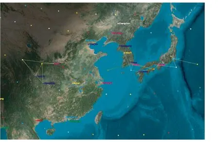
Fig. 1 The scene modeled by Starlink

3 Satellite-to-Ground Channel Formulation

The whole formulation is divided into two parts:the LSTM network part is for predicting the SNR, and the other part is for selecting the appropriate redundancy rate. This is described in detail in the following.

3.1 Satellite-to-Ground Channel SNR Prediction

Starlink is a famous satellite constellation established by SpaceX. 1 584 satellites are evenly distributed on 22 orbits, with 72 satellites in each orbit. The orbital inclination is 53 degrees, and the orbital height is 550 km. Satellites and ground equipment communicate while satellites move at high-speed, and SNR changes rapidly.Since the satellite-to-ground channel loss is mainly free space loss (FSL) and rain loss, the SNR at the next moment will be related to the SNR at the previous few moments. So we adopted the LSTM network, a kind of recurrent neural network, to predict SNR. The values of rain loss and real-time weather in different locations on earth differ, so we use latitude and longitude to represent the location of satellites and ground equipment in order for the network to learn a global SNR prediction model. When predicting SNR, the satellite can understand the weather conditions on the ground, the latitude and longitude information of the ground equipment, so it can determine whether to leave a margin for rain loss and what the margin should be. Since the single connection time is concise within 3 min, the FSL in a single connection is first smaller and then larger. After predicting the SNR at the next moment, the satellite can dynamically select the redundancy that can maximize the throughput based on this SNR. This saves valuable band resources to the greatest extent. In a nutshell, satellite use past information to predict SNR for next frame, and AMC is adopted to fully utilize channel. After the user receives the message, send the real-time SNR in the feedback message, as shown in Fig. 2.

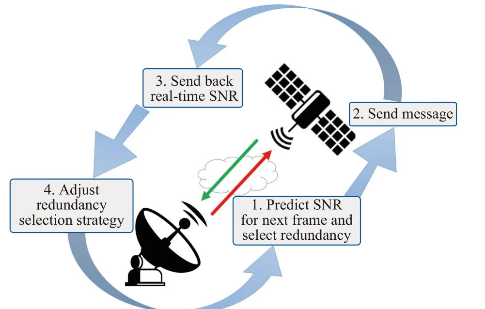
Fig. 2 The whole process of satellite-to-ground channel SNR prediction

After predicting the SNR at the next moment, we can dynamically adjust the code rate of the next frame. In practice, satellite communication uses the accumulate repeat-4 jagged-accumulate (AR4JA) [15, 16] code in the Consultative Committee for Space Data Systems(CCSDS) standard, which is a special low-density parity-check (LDPC) [17, 18] code. It has the characteristics of easy construction, simple storage, and low error floor, which is very suitable for satellite communication scenarios. In the case of good communication conditions, we can use a lower redundancy rate encoding method,and when the communication quality is poor, we can choose a more reliable high redundancy rate encoding method. This allows us to achieve maximum throughput under the premise of reliable communication.

3.2 Redundancy Selection

CCSDS is an organization that develops standards for space communications. Starlink has many technical indicators based on CCSDS, such as its communication frame format. According to CCSDS regulations, three code rates of LDPC codes can be used for LEO communications [19],which are 50%, 66.7%, and 80%, respectively.There are many ways to construct LDPC codes.As the computing power of satellites is precious,in this article, we use the AR4JA code recommended by CCSDS and dynamically adjust its redundancy rate to maximize throughput.

When constructing AR4JA code [4], we need to construct a cyclic matrix, which is constructed by accumulator and repeater, which is convenient, simple, and efficient. In addition, the minimum Hamming distance of the AR4JA code has a linear relationship with the code length,which makes up for the high error floor of ordinary LDPC codes [20]. The efficiency of encoding and decoding and energy consumption control is crucial for satellites.

CCSDS only provides three code rates but with the development of communication technology and quickly changing scenarios, we may need more code rates. As many as 28 coding schemes are stipulated in the satellite TV protocol, DVBS2 [12]. Therefore, we have additionally constructed AR4JA codes with three code rates to simulate more complex scenarios. The code rates we constructed are 33% and 60%, interspersed with the original code rate to simulate scenes with better or worse signals.

Since bandwidth resources are precious, we hope to transmit as much data as possible while ensuring the bit error rate (BER) and packet error rate (PER). Therefore, we hope to maximize throughput.

whereNis the number of bits per packet. When BER rises, PER rises rapidly. We approximate the PER curve as a discount model: when the FER is greater than 90%, it can be considered that all the sent packets have been correctly received; when the FER is less than 90%, we set that the probability that the information in the packet can arrive correctly is 0 [21].

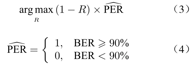
whereRrepresents the redundancy rate.

4 SNR Prediction and Dynamic Adjustment of Redundancy Rate

4.1 Traditional Time Series Forecasting Methods

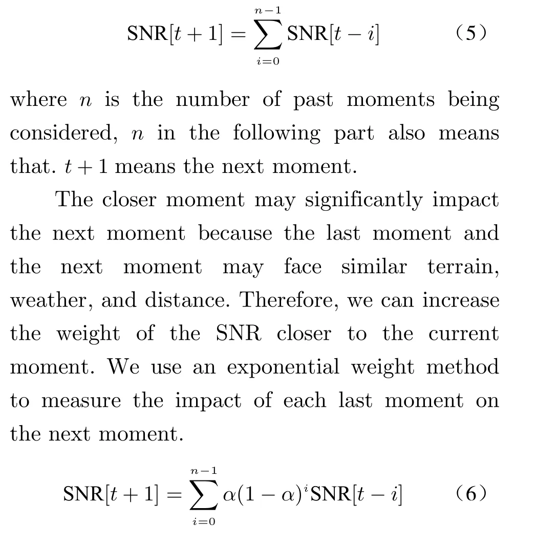
It is complicated to accurately predict the SNR of satellite-to-ground channels with rapid changes, long distances, and large RTTs. From the precious, we can know that the SNR of the satellite-to-ground channel at the current moment is related to the past few moments. The most straightforward idea is to use the average SNR of the last few moments. Generally speaking, a simple linear average can yield good results.

4.2 Time Series Prediction Based on Machine Learning

The traditional method is usually based on the past SNR information to estimate the SNR at the next moment. Still, we can get more details than this: we can roughly know the local rain loss intensity from the latitude and longitude, and the position and speed of the satellite at the next moment can be calculated from the satellites’position in the last few moments. We can consider more information and extract the practical part to help us predict the SNR.

SVR is an application of support vector machine (SVM) to regression problems. When using SVM, we need to use the kernel function to map the data to the feature space and then build a linear classifier in the feature space. When using SVR, we first map the data to the feature space and then fit it with a high-dimensional straight line. Since SVR has no memory, it can only predict the SNR at the next moment based on external information. Let the inputxof SVR be a four-dimensional vector (sunny, rain, fog,distance) in our experiment. In addition, the training time using SVR for all the data is too long due to the large amount of data. Finally,because the rain loss varies significantly between different cities, the training effect is not good.Therefore, we chose to train separately for each city and achieved good results.

LSTM network is a kind of recurrent neural network (RNN), which has internal gates to adopt past information. These three gates are the forget gate, input gate, and output gate, which determine the degree of influence of the previous and current information on the future. Thanks to the development of computing power in recent years, we can perform parallel computing on the GPU, which significantly improves the efficiency and allows the LSTM network to process data from all cities without taking too long. The LSTM network model we constructed is divided into five layers, as shown in Fig. 3.

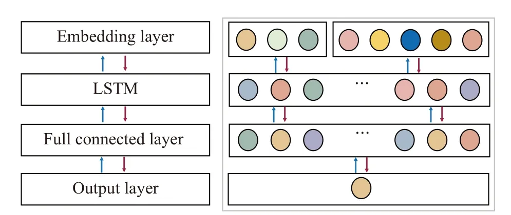
Fig. 3 Structure of LSTM network

The first layer is the input layer. As the LSTM network has more powerful information processing capabilities, we split the distance,which is one of the inputs of SVR, into the latitude, longitude, and height of the satellite in the actual scene. Moreover, there are eight dimensions in the input layer. The second layer is the embedding layer, and we separate weather information and distance information into two parts.It turns out that processing data at the beginning of the network helps the network to converge. The third layer is the LSTM layer, which has a depth of 1 layer and contains 100 hidden neurons. This layer is the network’s core, which can learn past information. The fourth layer is a fully connected layer, which is used to connect the output of the LSTM layer and the last layer.There are also 100 neurons in this layer. Finally,the last layer is the output layer with only one neuron. There is a Relu layer as activation functions between the third and fourth layers and the fourth and fifth layers.

5 Experiment

5.1 Dynamic Adjustment of Redundancy Rate

We use the method mentioned in Section 4 for simulation. Too largenwill make noise into consideration, while too smallnwill cause the model to fail to learn the data laws thoroughly. In addition, we experimented with the value ofαfrom 0.1 to 1 in the exponential average.

In the SVR experiment, we trained separately for each city. Since SVR has a variety of kernel functions, we selected three of the most commonly used kernel functions[22]: linear kernel, polynomial kernel, and RBF kernel. In the experiment, the data was shuffled first, and then 70% of the data was used as the training set and 30% as the test set.

The input data of the LSTM network is segmented, and we treat the data of a single connection as a whole piece of data. In LSTM network training, we tried different network layers, but the results proved that more LSTM layers would only bring more noise, so we chose a single-layer LSTM network, and the number of neurons was set to 50. In training, we set the learning rate to 0.01 and the batch size to 128. During training,we used a strategy of gradually reducing the learning rate to fine-tune the model. For example, in 400 epochs of training, we multiply the learning rate by 0.1 at 100 and 200 epochs. We chose Adam as the optimizer and mean absolute error (MAE) as the measure of loss. We have tried to mean square error (MSE) and MAE during training but found that MSE will decline very slowly after it drops below 1. Furthermore, tend to get errors with little difference, while MAE tends to get sparse errors, which is also mentioned in [3]. In the training of the LSTM network, we use 70% of the dataset as the training set, 20% as the validation set, and 10% as the test set.

After obtaining the SNR, we need to select the redundancy rate dynamically frame by frame.At the farthest distance of 794 km, the RTT of LEO is 5.3 ms, and when the satellite is directly above the ground equipment, the RTT is 3.6 ms,this duration is not perceivable by humans, so we assume in the lab that the satellite will send the following data only after receiving the previous one, This means that the satellite can receive the position information of the ground equipment and the SNR of the previous one. We can choose the best redundancy rate using the SNR of the precious moments, the location, and the weather information we just received.

5.2 Result

We selected a total of different methods for predicting SNR: linear smoothing(LS), exponential smoothing(ES), SVR, and LSTM. MAE was chosen as the metric for judging the performance in the experiments.

As shown in Fig. 4 and Tab. 1, the stability of both linear smoothing and exponential smoothing is high. The MAE of linear smoothing is around 0.1, while exponential smoothing is around 0.06. This is because exponential smoothing takes more into account the closer moment.Moreover, the closer moment is more similar to the next moment because the satellite moves linearly. Resulting in its next moment’s position and velocity being more similar to the previous moment, due to the short time, the satellite-toground channel and rain loss are similar to the last moment.

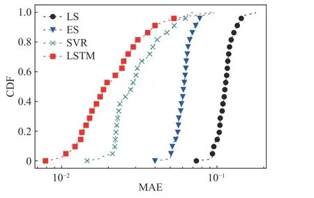
Fig. 4 Cumulative distribution function (CDF) of MAE for different methods

Tab. 1 MAE of different methods

The MAE of SVR is about 0.03, but one city has an MAE of 0.7, which shows that SVR does not always learn the characteristics of each city accurately, especially the cities with variable weather near the equator. The LSTM method results are satisfactory, with a mean MAE of 0.024 and no great ups and downs. Even in the worst part, the results are similar to those of the SVR. The loss curves during training are shown in Fig. 5.

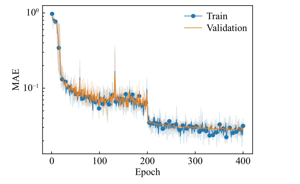
Fig. 5 The loss curve of the LSTM network during training

The loss of the validation set is in line with the trend of the training set, which proves that the LSTM network is not over-fitted. The loss decreases significantly at the 200th epoch and becomes smooth due to the reduced learning rate.In addition, the LSTM network has an advantage: while the other four models model cities individually, the LSTM network works in a standard model for the whole world. This avoids sudden changes when switching between city models and eliminates the difficulty of thinking about how the models should be switched. On satellites,where storage and computational resources are scarce, the size of a single LSTM network model is only 170KB. In contrast, other methods such as SVR have to store multiple models for different regions. Avoiding switching between models will also save some time.

Each SNR has a corresponding optimal redundancy rate that maximizes throughput, and our goal is to select as many of these optimal redundancy rates as possible. Our experiments consider that the FDR is greater than 90% for all correct reception and more petite than 90% for all incorrect reception. In order to quantitatively compare the performance gap between different methods, we define the optimal match ratio(OMR) as

Where the equation’s numerator is the result of choice based on the predicted SNR according to the maximization throughput principle, and the denominator is the optimal throughput. The location where the non-optional redundancy rate is chosen usually occurs at the junction of the two redundancy rates. This is due to the difference between the predicted SNR and the actual SNR, resulting in a non-optimal redundancy rate.Therefore it is essential to predict the SNR accurately.

As shown in Fig. 6 and Tab. 2, the OMR of linear and exponential smoothing is around 98%,and the effect of this simple method is good when the interference is not substantial. The results of both SVR and LSTM are good, and from Fig. 6 we can see that LSTM is more stable in coding scheme selection, and the OMR of several cities in SVR is low, which means that SVR is not enough to learn the SNR characteristics of all cities accurately.

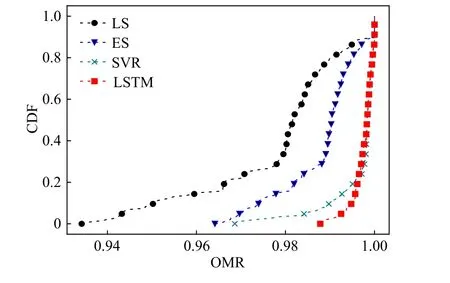
Fig. 6 CDF of different methods of OMR

Tab. 2 OMR of different methods

6 Conclusion

In this paper, we model the parameters of the Starlink satellite constellation to simulate the communication between LEOs and ground equipment. In the modeling, we consider various factors, including free-space loss, rain loss, ionospheric loss, etc., to simulate the communication scenarios. We used the top cities globally in terms of GDP as ground stations and simulated them communicating with the satellite. To fully consider the impact of weather and cloud cover on SNR, we use 24 h of weather data in a day to simulate the satellite-to-ground channel under actual weather.

After the modeling was completed, we utilized different methods for SNR prediction. These methods are divided into machine learning methods and traditional methods. Traditional methods include linear, exponential, and machine learning methods, including SVR and LSTM.Since the LSTM network can consider past information and utilize it, it works best and predicts the most accurate SNR. SVR also works well,but it cannot learn its features accurately in some cities with fast-changing weather.

After obtaining the predicted SNRs, we select the redundancy rate of AR4JA coding based on the SNRs and compare it with the best redundancy rate. The best redundancy rate is the one that maximizes the throughput at the current SNR. In our experiments, we adjust the redundancy rate frame by frame. Moreover, the LSTM network can predict the value of the next frame by the SNR returned from the previous frame making full use of the historical information. The experimental results show that the redundancy rate is easily miss-elected at the edge of redundancy rate switching. Since the LSTM network predicts the satellite-to-ground channel accurately, the LSTM network has the highest OMR.