An overview of quantum error mitigation formulas

Dayue Qin(秦大粤), Xiaosi Xu(徐晓思), and Ying Li(李颖)

Graduate School of China Academy of Engineering Physics,Beijing 100193,China

Keywords: quantum error mitigation,quantum computing,quantum error correction,noisy intermediate-scale quantum

1. Introduction

Quantum computers have the potential of outperforming classical computers in solving certain problems.[1]With a particular problem, one needs to map a quantum algorithm into quantum circuits that the quantum hardware can execute.However,the quantum state stored in any physical system,no matter superconducting qubits,trapped ions,etc.,[2]has a limited life time due to interactions with the environment. Besides,any operation is associated with noise. These altogether lead to unreliable computing outcomes. For superconducting qubits, the error rate per two-qubit gate, i.e., the probability of an error occurring in the gate, is about 0.5% with current technology.[3]The error rate limits the number of quantum gates in a circuit,to merely a thousand.[4,5]Therefore,it is necessary to minimize the impact of noise in a quantum circuit,generally by the means of quantum error correction(QEC)or quantum error mitigation(QEM).

QEC is the conventional method to correct errors by taking the use of quantum error correction codes. Quantum states are encoded into some code space,which is a subspace of the entire Hilbert space - physically, a logical qubit is encoded into several physical qubits. The encoding,error detection and correction are realized with quantum gates that are also noiseprone. Therefore, if the physical error rate per gate is higher than a certain threshold, performing error correction can introduce more errors than that it can correct.[6]QEC also requires an overhead cost on qubits for encoding the logical information. For example,when the physical error rate is 10-3,about 1.4 million qubits are required to calculate the electronic structure of 54 spin-orbitals using the surface code.[7]With the current technology,it is still challenging to experimentally demonstrate beneficial error correction in quantum computing.

As the name suggests, QEM methods are designed for mitigating the effect of errors instead of correcting them.They can work in a quantum circuit with an error rate higher than the threshold of QEC, without the large qubit overhead. Therefore, QEM is suitable for quantum devices in the noisy intermediate-scale quantum (NISQ) era,[8]a midway towards fault-tolerant quantum computers[9]in which quantum computing is fully protected by QEC. NISQ devices have only dozens to hundreds of qubits, nevertheless,they have demonstrated the quantum advantage on a specific problem,[4,10]and it is believed that they can retain this advantage to solve practical problems. To achieve this goal, many quantum algorithms[11,12]have been proposed. Incorporating QEM methods is essential for certain applications on NISQ devices.

Various QEM methods have been proposed. In methods such as error extrapolation(or zero-noise extrapolation)[13,14]and probabilistic error cancellation (PEC),[14,15]given some knowledge about the noise, we can compensate errors and make the computing result closer to the true value. These methods do not require additional qubits. The knowledge of the noise, e.g., a parameter such as the error rate or a concrete error model, can be obtained with some characterization methods.[16,17]Alternatively, the parameters used in QEM protocols can be optimized in a learning-based or datadriven manner.[18,19]In symmetry verification[20,21]and virtual distillation,[22-25]errors are eliminated based on certain constrains on the quantum state,i.e.,symmetry and purity,respectively. Multiple copies of the noisy state are required for effectively increasing the purity in virtual distillation. These methods are more similar to QEC than error extrapolation and PEC:In a QEC code,a symmetry(i.e.,the stabilizer group in stabilizer codes) is constructed at the cost of qubit overhead.In addition to general-purpose QEM methods, protocols are also developed for specific algorithms.[26-28]For example,the quantum subspace expansion[26,27]is a protocol designed to reduce errors in a variational quantum eigensolver.[29]

In this paper,we summarize the state-of-the-art error mitigation methods. Although they work in different ways, we formulate them in a general form. In this way, we explicitly define two characteristic quantities of all QEM protocols, the bias and the variance. With the general form, there is a universal way to combine different protocols and optimize them in the leaning-based manner. In Section 2, we introduce the notations and the general form. QEM methods are specifically described and discussed from Section 3 to Section 7. We introduce the Clifford-circuit learning method in Section 8 and summarize the combined methods in Section 9. A summary is given in Section 10.

2. Notations

where(λ1,λ2,...)are the parameters. The formulaFas well as the choice of (C1,C2,...) depend on the error-mitigation method. Different error mitigation methods employ different techniques to determine the parameters in the formula.

We characterize an error mitigation method with two quantities, the bias and the variance. In quantum computing,yCis estimated with the random outputs of the circuitC. We denote the estimator ofyCwith ˆyC. Usually, ˆyCis unbiased,i.e., E[ˆyC]=yC, and the variance depends on the number of circuit executions. For example, if the observableO=Zis the Pauli operator of a qubit,the measurement outcome of one circuit execution is a random number±1. According to the empirical mean estimator, ˆyCis the average value of measurement outcomes, and its variance is (1-y2C)/M, whereMis the number of circuit executions. Given ˆyC, the estimator off＇Cis ˆf＇C=F(ˆyC1,ˆyC2,...)according to the error mitigation formula.Bias and variance of the QEM estimator are respectively E[ˆf＇C]-fCand E[ˆf＇2C]-E[ˆf＇C]2. In some error extrapolation protocols and PEC,the formula is linear inyC,thus E[ˆf＇C]=f＇Cif each ˆyCis unbiased, and the bias of the QEM estimator isf＇C-fC; in general this result on the bias does not hold.Usually,error mitigation can reduce the bias while increasing the variance, in comparison with the raw quantum computing without error mitigation(corresponding tof＇C=yC). The schematic diagram of error-free,erroneous and error mitigated computation results can be found in Fig.1.

3. Error extrapolation

In error extrapolation, the basic routine is to execute the quantum circuit at various noise levels and then extrapolate to the zero-noise limit. The two essential components are extrapolation formulas and error-boosting methods. Errorboosting methods increase the error rate while preserving the error model. With the computation results at increased error rates,we can predict the error-free result according to the extrapolation formulas.

3.1. Polynomial extrapolation

The idea of error extrapolation was introduced in works by Li and benjamin[13]and Temmeet al.,[14]in which the polynomial fitting function is considered. It is assumed that the erroneous result can be expressed with the polynomial decomposition

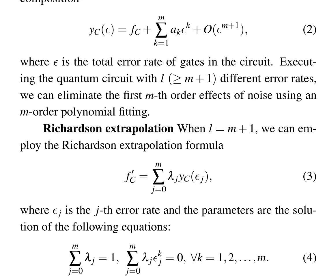
Truncated Neumann series Recently, Wanget al.[30]proposed error mitigation with truncated Neumann series. In this protocol,a formula resembling that in Eq.(3)is used,but the parameters are determined according to the truncated Neumann series. LetF:E →R be a linear map from a superoperatorE,which is a squared matrix in the Pauli transfer matrix representation,[17]to the real field R. Under the condition of limk→∞(I-E)k=0, which can be satisfied if‖I-E‖＜1 in some consistent norm,it holds that

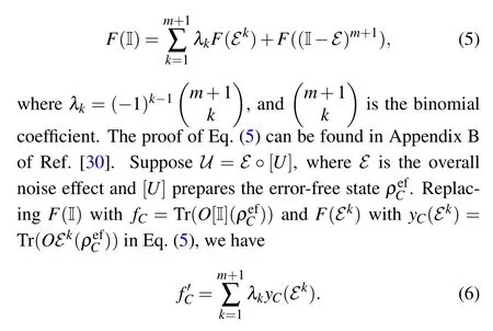
HereyC(Ek) can be realized by repeatedly applyingEforktimes. The bias in Eq. (6) decays exponentially withkwhen the error rate is small.

3.2. Exponential extrapolation

In some cases,the exponential extrapolation proposed by Endoet al.[15]has advantages in accuracy. The simplest exponential extrapolation is

given two error rates∊0＜∊1. Giurgica-Tironet al.[31]summarized the extrapolation formulas and introduced a more general form of poly-exponential extrapolation,in which the logarithm of erroneous result fits to a polynomial function. Cai[32]generalized error extrapolation to the multi-exponential functions where the sum of exponents is the fitting function.

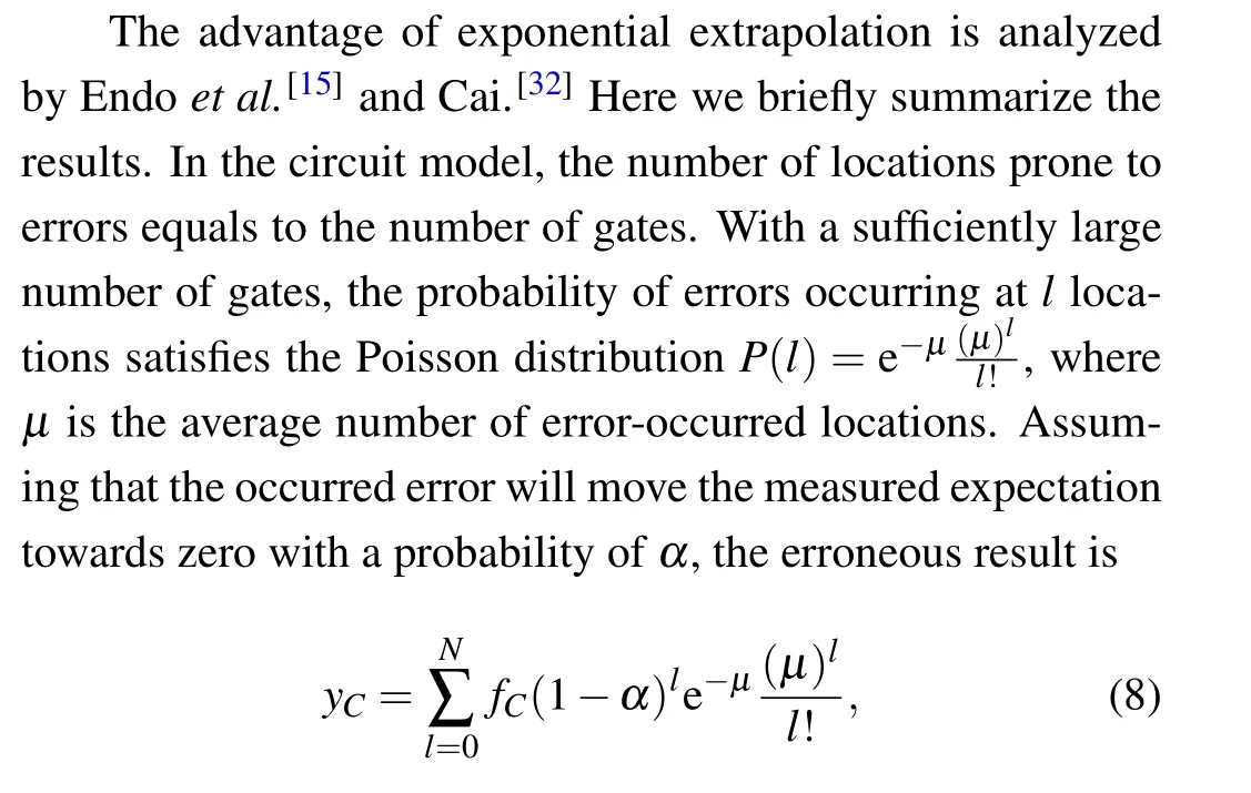
and in theN →∞limit it becomes an exponential functionfCe-µα. The advantage of exponential extrapolation is numerically demonstrated in Refs.[15,31]. Observations of the fidelity decay in experiments,e.g.,the results in Ref.[33],also support this conclusion.

3.3. Resource cost

Here we briefly discuss the resource cost of error extrapolation. We take Richardson extrapolation as an example. One may think that we can arbitrarily improve the precision by increasing the extrapolation ordermin Eq.(2). This is true only when we can exactly measure the value ofyC(∊), which is impossible because of the shot noise. In fact, if the extrapolation curve interpolates all the data points, such as that in Richardson extrapolation, the variance is increased by a factor around ∑mj=0λ2j. Therefore,we should in practice choose a proper extrapolation orderm. Krebsbachet al.[34]studied the variance-bias trade-off in Richardson extrapolation and proposed the optimal extrapolation orderm, spacing|∊j-∊j-1|for each noise rate given the overall sampling overhead. From the perspective of statistics,the increased variance is referred to the phenomenon of overfitting,[35]which can be suppressed with increased number of data pointsl(≫m) and by using fitting methods such as least squares rather than Richardson extrapolation.

3.4. Error-boosting methods

The first method takes use of Pauli twirling and random Pauli gate insertion.[13]This method relies on the assumption that quantum errors of the single-qubit gates can be ignored comparing with those of multi-qubit gates. We can effectively increase the error via randomly inserting Pauli gates after each multi-qubit gate. Pauli twirling converts an arbitrary noise channelEiinto Pauli noise:[36]

whereσi,σj ∈{σI,σx,σy,σz}are single-qubit Pauli operators andσiσjdenotes a tensor product.Pi jare positive coefficients satisfying ∑i,j Pi j=1. To implement the Pauli twirling technique, we randomly insert Pauli gates before and afterUi, resulting in[σdσc]°Ui°[σbσa], whereσaandσbare uniformly sampled from{σI,σx,σy,σz}and accordinglyσdσc=[Ui]σbσa. To boost up the error rate, a further step is to randomly insert Pauli gates after each multi-qubit gate. Recall Eq.(9)and assume a small error rate,randomly inserting each Pauli gateσiσjwith a probability ofrPi,jcan boost the error rate from∊to(1+r)∊.

The second method is to insert identity-equivalent gates.The approaches to this end include repeating self-invert gates for odd times,[37,38]gate folding[31]and identity insertion.[39]Typically,this method is based on

for arbitrary unitary operator ˜Uand non-negative integerr.Gate folding according to the above equation will amplify the error rate by a factor of 1+2rif the noise operation commutes with the unitary operator and the error rate is small.To be more detailed, suppose the noise operation on thei-th gate is in the form ofEi=(1-α)[I]+αNi,the noise operation on the folded gates isEri=(1-r＇α)[I]+r＇αNi+O(α2),wherer＇=1+2r. Here we have assumedNicommutes with ˜U. In the case thatαis small, the error rate is enlarged by a factor of 1+2r. Primitively, we should fold every erroneous gate with the samer, such that the error model is unchanged. In that case,we can only amplify the total error rate for 1,3,5,...times. To achieve denser spectrum of error rates,we can choose to foldmout ofNgates and the error rate is increased by a factor of 1+2rm/N. Be aware of that partially folding a circuit may not only increase the total error rate but also severely change the error model, thus it should be subtle when choosing which gate to be folded. To keep the error model as unchanged as possible, Giurgica-Tironet al.[31]divided the quantum gates into subsets and chose to fold particular gates in each of the subsets.Heet al.[39]used the method of random identity insertion. They setrof each gate as a random variable and sampled circuits according to the distribution ofr.Recently,Schultzet al.[40]introduced the method of gate Trotterization. They proposed compiling a gateGinto products of several gates according to the formulaG=(G1/r)r.

The third method is stretching the Hamiltonian. On realistic quantum hardware, quantum gates are implemented by evolving qubits’ state under a controlled time-dependent Hamiltonian denoted byH(t). The stretched HamiltonianH(t/r)/rcan increase the error rate by a multiplicative factor ofrunder the assumption that the noise generator is independent of the Hamiltonian and constant in time.[14]In experiments,we can realize the stretched Hamiltonian by reducing the pulse strength that controls the qubits while prolonging the pulse time. An illustrative example is, similar to the Rabi stretch for single-qubit in Ref. [41], a spin initialized in theZ-direction evolving under aX-direction magnetic fieldH=Bσx(t). The method of stretching the Hamiltonian here is to increase the durationtand reduce the field strengthBby the same multiple. A more practical example is given in Ref.[42],where it tunes the cross-resonance pulse on a superconducting quantum processor.

Here we briefly discuss the advantages and disadvantages of these three error-boosting methods. The first method requires accurate understanding of the error model, and the error rate is boosted in a pseudo manner, i.e., the error rate is not actually increased but the collective result of random circuits is equal to the result on an error-increased device. The advantage is that, with the aid of reliable gate benchmarking methods such as gate set tomography,[17]the critical condition that boosting error will not change the error model can be fulfilled. The second method is easy to implement. Comparing with the first one, the second method does not need any definite knowledge about the noise model. However,it is at greater risk that the error model is changed when folding gates. This is not a serious problem when with only simple error models such as depolarizing. In general, it may cause that, quoted from Ref. [5], “arbitrarily deviate from the desired result when only slightly more complicated error models are considered”. Both the first and second methods are in the digital level and friendly to cloud-platform users, while the third method requires direct control of the underlying quantum hardware. Nevertheless, pulse-level control is accessible through some hardware providers.[43,44]As shown in the work of Schultzet al.,[40]the amount of increased noise by different methods depends on the time-correlation. The performance of different methods is similar with white noise, but can be significantly different for time-correlated noise.

3.5. Multiple noise parameter extrapolation

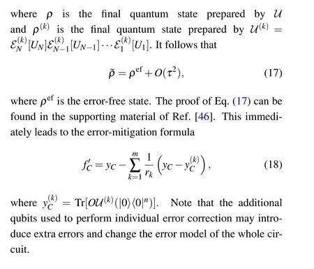
Hyper-surface fitting[45]and error mitigation via individual error reduction[46]are proposed by Otten and Gray. Both works considered the linear error mitigation formula with multiple noise parameters.

4. Probabilistic error cancellation

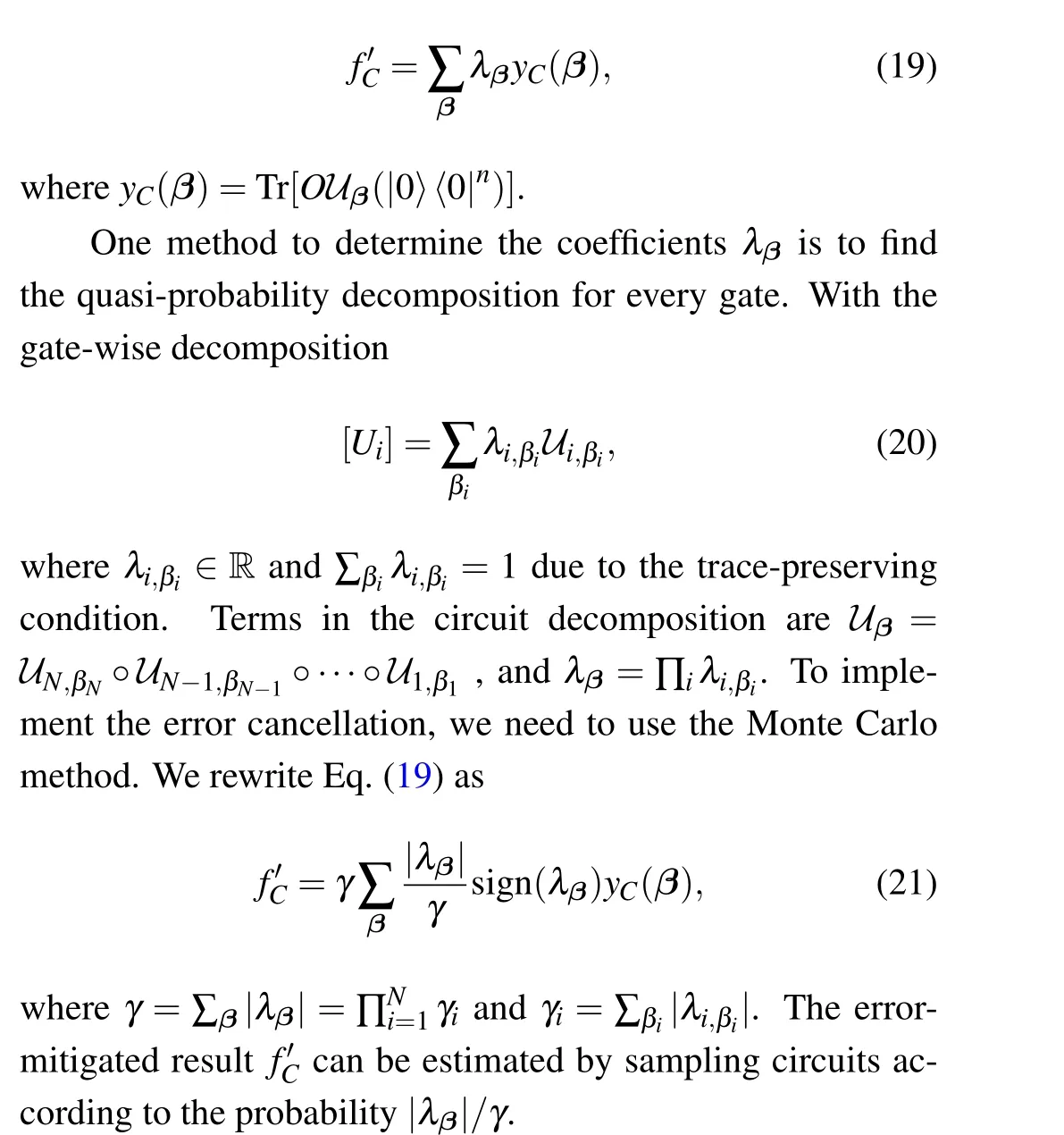
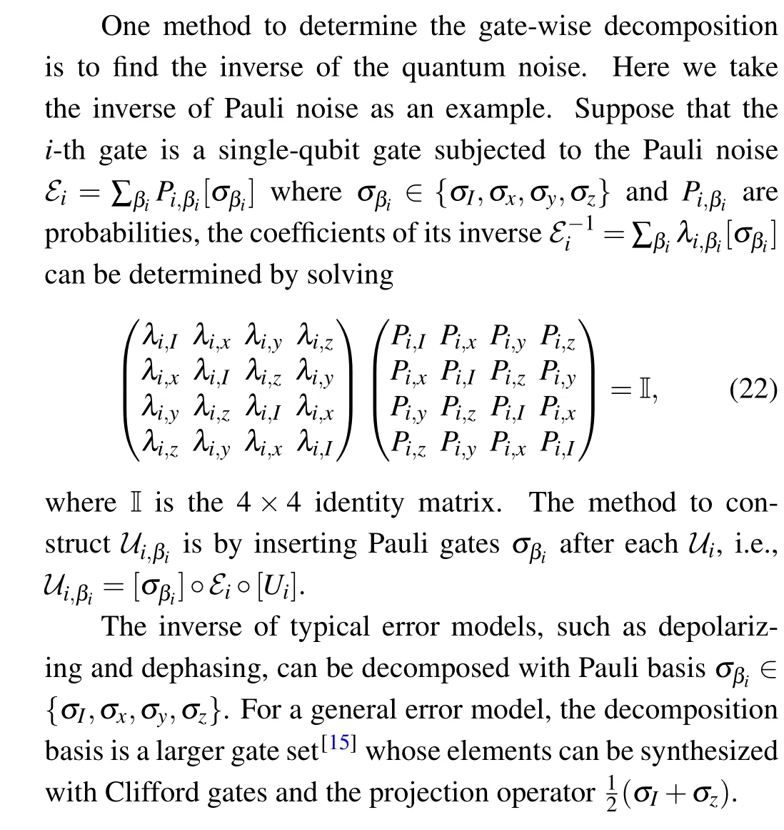
Probabilistic error cancellation (PEC) was proposed by Temmeet al.,[14]which is implemented based on a quasiprobability decomposition. A practical method of constructing the formula using gate set tomography and universal gate set was introduced by Endoet al.[15]The basic idea is that an error-free operation can be expressed as a linear combination of erroneous ones. Suppose that the vectorβ=(β1,β2,...,βN) specifies a quantum circuit (βispecifies thei-th gate) and there exists a circuit decomposition [Uβ] =∑β λβUβ,the error cancellation formula is

4.1. Resource cost

The sampling overhead of PEC is determined byγ. In comparison with the case without error mitigation, the variance in PEC is increased by a factor ofγ2: if we use Monte Carlo estimation according to Eq.(21),we needγ2times more circuit executions in order to achieve the same variance as in the error-free case. Recall thatγ=∏Ni=1γi,the sampling overhead increases exponentially with the number of gatesN.Considerγi=1+O(∊/N)and ∏Ni=1(1+∊/N)≈e∊where∊is the total error rate,PEC is efficient when∊is small.

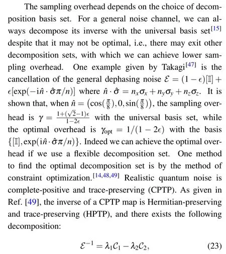
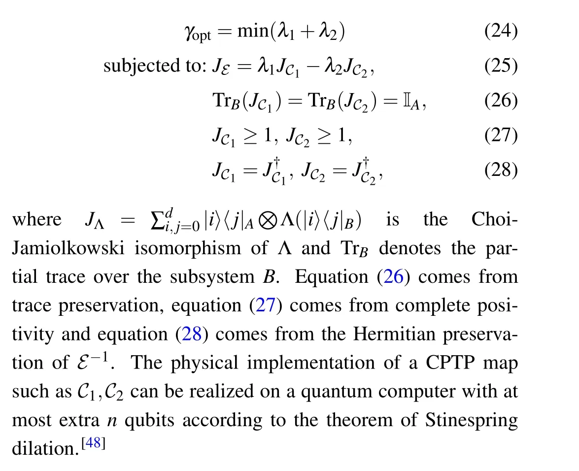
whereE-1is a HPTP map,C1,C2are CPTP maps,andλ1,λ2≥0 are two real numbers. According to Eq.(23),we can employ the following constraint optimization to determine the optimal resource cost:

4.2. Continuous-time formalism

Sunet al.[50]proposed the stochastic PEC, which extends the formulism of PEC for analogue quantum computation, such that the PEC protocol can be engineered at the pulse level and attain extra resilience against gate dependence and non-local noise effects. Stochastic here means randomly choosing time points to add correction operation instead of checking everywhere. We for now modify our notations to adjust to the continuous time formalism. Other than the total number of gates, we here considerN=T/δt, whereδtis a small time interval andTis the time when the final state is prepared. During thei-th time interval, the time evolution on a realistic quantum machine is

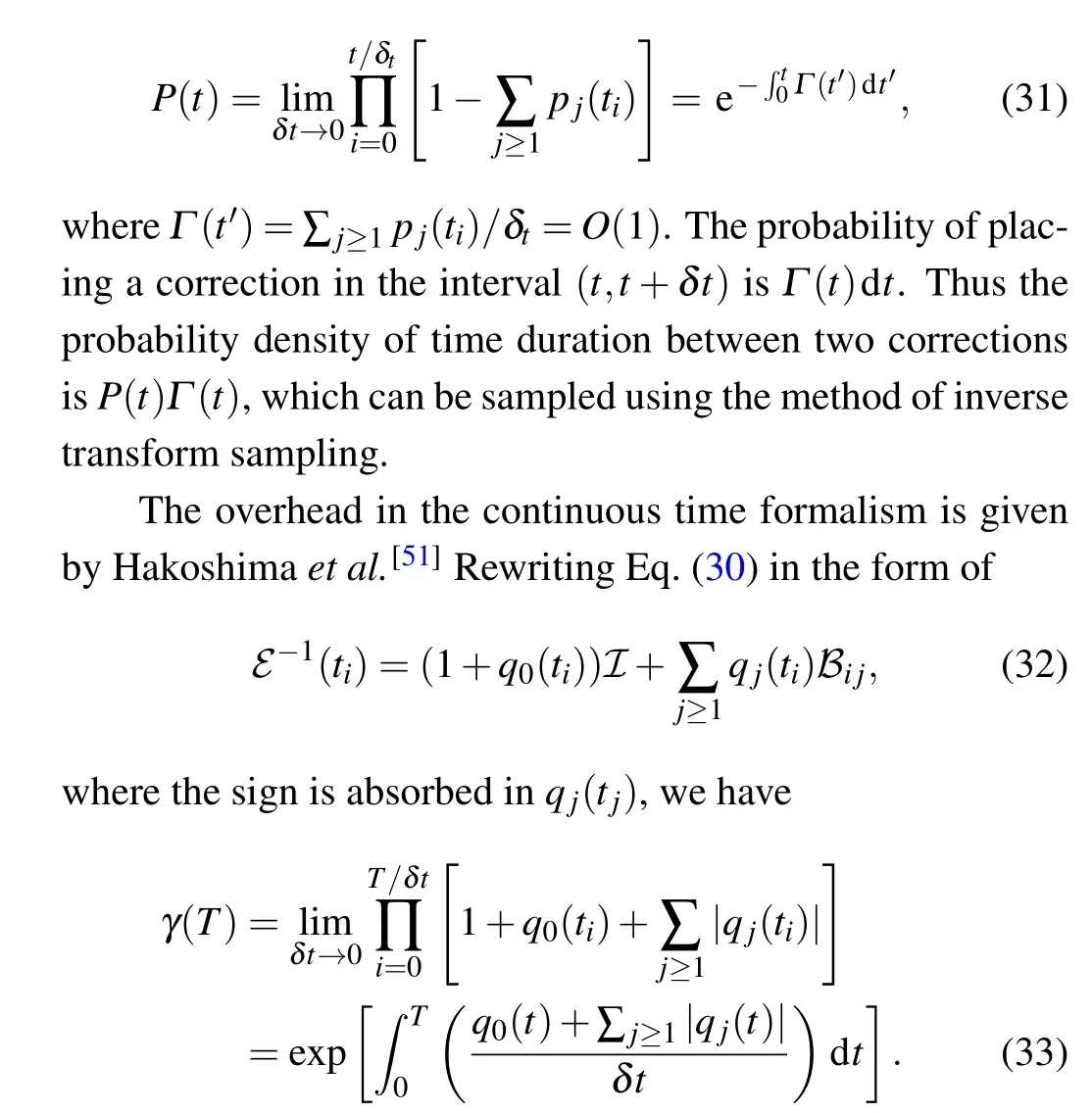
The above equation enables us to investigate the role of non-Markovian noise played in the resource cost of PEC.Hakoshimaet al.[51]demonstrated that non-Markovianity can reduce the PEC resource cost.

5. Mitigating measurement error

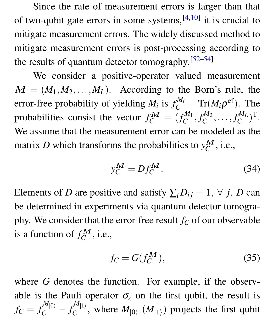
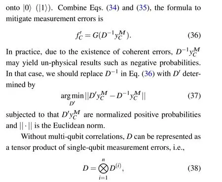
whereD(i)describes the measurement error on thei-th qubit.When there are correlated errors, we should employ efficient methods featuring these correlations.[55,56]

6. Virtual distillation

Recently, various virtual distillation (VD) methods were proposed in several works. We categorize these methods into two kinds: the multi-copy approach[22,23]and the state verification approach.[24,25]

Given an erroneous stateρ,the purified stateρM/Tr(ρM)has exponentially reduced errors. Suppose we have the following spectrum decomposition of the erroneous state:where the observableOis on one of the copies andS(M)is the cyclic permutation operator, i.e.,S(M)|ψ1〉|ψ2〉···|ψM〉=|ψ2〉|ψ3〉···|ψ1〉. We can verify Eq.(42)by explicitly writing both the left-and right-hand sides into summations of matrix entries,while here we provide an intuitive interpretation given by Koczor.[22]Suppose there areM=2 copies of states prepared as|ψ〉|ψ〉.If any one of the two copies is flipped(due to an error) to an orthogonal state|˜ψ〉, measuring the operatorOS(2)will yield〈ψ|〈˜ψ|OS(2)|ψ〉|˜ψ〉=〈ψ|O|˜ψ〉〈˜ψ|ψ〉= 0,thus the contribution of the error vanishes in the purified expectation. To compute the right-hand side of Eq.(42),we can prepareMcopies of the erroneous state and measure the expectation ofOS(M). To measure the expectation,one approach is measurement by diagonalization,[23]i.e.,we can append extra gates to the end of the original circuit to transformOS(M)into a sum of measurable observables. The transformation procedure is practical when the number of copiesMis small,sinceS(M)can be represented as tensor products of qubit-wise permutation operators which lies in 2M-dimensional Hilbert space. The other way to measure the expectation ofOS(M)is by utilizing the Hadamard-test technique.[22,59]We here provide an example circuit[22]in Fig.2

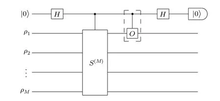
Fig. 2. An example circuit to implement VD via the Hadamard-test technique. The qubit on the top is the ancilla. M copies of quantum states ρ1,ρ2,...,ρM are prepared in parallel on the left. The controlled-S(M) gate can be decomposed into M-1 controlled-SWAP between states. The numerator in Eq. (41) is computed as Tr(OρMC )=2P(0)-1, where P(0) is the probability that the output state of the ancilla is|0〉. The denominator in Eq.(41)is computed as Tr(ρMC )=2P＇(0)-1,where P＇(0)is the probability without the controlled-O gate in the dashed box.

The state verification approach is to check whether or not the dual form of the state-preparation circuit can evolve the state back to its initial. We call this procedure the dual test.In practical quantum computation, the expectation of an observable is measured by averaging over many circuit executions. State verification only keeps those executions that pass the dual test and discards the rest. The state-verified circuit usually has an intermediate measurement sandwiched between the state-preparation circuit and its dual circuit. The intermediate measurement can be executed in a non-destructive manner with the aid of one auxiliary qubit. We here provide an example circuit[25]in Fig. 3. The multi-copy approach and state-verification approach can be combined[60,61]to achieve qubit overhead lower thannM+1.

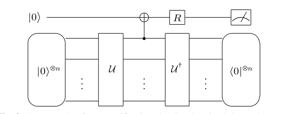
Fig.3. An example of state verification circuit. The circuit is used to compute f＇ =Tr(σzρ2)/Tr(ρ2), where ρ =U(|0〉〈0|⊗n) and σz is the Pauli-Z operator on the first qubit of ρ, i.e., the control qubit of the CNOT gate in this figure. The qubit on the top is the ancilla and the Pauli-Z (-X)operator on the ancilla is denoted by σ(a)z (σ(a)x ). R can be either I or H. When R=I,we measure 〈σ(a)z 〉 of the ancilla. When R=H, we can effectively measure 〈σ(a)x 〉 of the ancilla by measuring in the Pauli-Z basis. The distilled result is f＇=〈σ(a)z 〉0/(1+〈σ(a)x 〉0),where〈O〉0 denotes the expectation of O conditioned on the output state being|0〉⊗n.

Here we briefly discuss the efficacy of VD. The variance is increased by VD due to the denominator Tr(ρM)＜1.Additionally, extra circuit executions are required in practical implementations. Firstly, measurement by diagonalization may mapOS(M)to the sum of several observable that can not be measured at the same time. We may have to estimate each observable individually and thus more circuit executions are needed. Secondly,state verification requires more circuit executions due to the discarding of failed trials in the dual test. The bias in VD comes from two aspects. One is due to the finite number ofM, however this part of bias can be exponentially suppressed by increasingM. The other one is due to the so-called coherent mismatch[22,62]or the noise floor,[23]i.e., the difference betweenρefand|ψ0〉〈ψ0|:Δ=1-Tr(ρef|ψ0〉〈ψ0|). Suppose thatρ=(1-∊)ρef+∊ρe,the coherent mismatch vanishes only if [ρef,ρe]=0. Given in Refs. [23,62], for general states and observables, the bias caused by coherent mismatch is bounded by

where||O||∞is the largest absolute eigenvalue ofO.

7. Symmetry verification and subspace expansion

Symmetry verification and subspace expansion are used to mitigate errors in the simulation of quantum systems.When the simulated system exhibits certain symmetries,we can mitigate errors by verifying these symmetries.[20,21]In quantum subspace expansion,[26,27]we can express the Hamiltonian in an effective subspace spanned by a set of noisy quantum states and obtain the error mitigated ground energy via generalized matrix diagonalization.

7.1. Symmetry verification

A symmetry is a unitary operatorSthat commutes with the system’s HamiltonianH,i.e.,SupposePSis the operator that projects into the subspace of symmetryS, i.e., the subspace with the right eigenvalue ofS. By measuring and post-selecting those states that pass the symmetry check ofS,[20,21]we can project the erroneous stateρonto

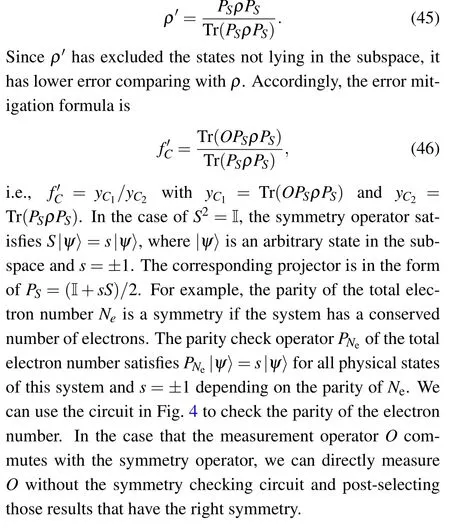
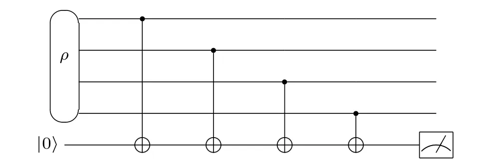
Fig. 4. A symmetry verification circuit for parity check. The qubit at the bottom is the ancilla. If spin-orbitals are mapped to qubits with |1〉 (|0〉)representing occupied(unoccupied)by an electron,we can check the parity of electron numbers by measuring the ancilla.

7.2. Quantum subspace expansion

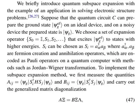
whereAandBare matrices with respective entriesAijandBij,Λ=diag(Λ1,Λ2,...,Λi,...)is a diagonal matrix of eigenvalues Λi,and Ξ is the matrix of eigenvectors. The error mitigation formula for the ground state energy is

7.3. Symmetry expansion

Symmetry expansion[63,64]can be regarded as the general form of symmetry verification and subspace expansion using symmetry operators for expansion. The complete symmetry group of an error-free quantum state is the stabilizer group S.Define the projector

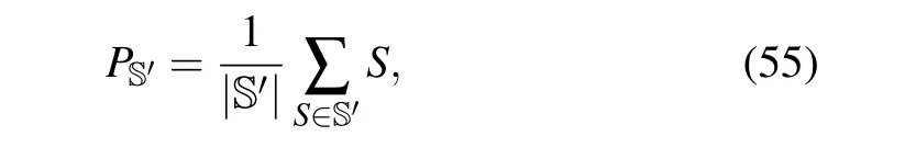
where S＇ ⊆S is a subset of the whole stabilizer group. If we choose S＇={I},PS＇means no projection and error is not mitigated. If we choose S＇=S, the noisy state is projected onto the intersections of all subspaces of symmetries which contain only the error-free state, and the error-free result is obtained.The practical choice of S＇in the NISQ era, is to let S＇be the intersection between the Pauli group and the stabilizer group,hence symmetry expansion is reduced to verify the Pauli operator symmetries.

8. Error mitigation using Clifford-circuit learning

The Clifford-circuit learning method was proposed by Strikiset al.[18]and Czarniket al.[19]Generally speaking, given an error mitigation formulaf＇C=F(yC1,yC2,...,λ1,λ2,...),Clifford circuit learning obtains the parameters by minimizing the loss function

where〈·〉C∈Rdenotes average over the set R,and C are training circuits generated by randomly replacing all non-Clifford single-qubit gates in a circuit with Clifford gates. Here we have assumed that all multi-qubit gates are all Clifford. In Eq. (56),f＇C＇can be computed on the noisy quantum computer according to the formulaFandfC＇can be computed on a classical computer utilizing the efficient simulation of Clifford circuits.[65]

In principle,we can take any form for F.Strikiset al.[18]took the form of PEC in Eq.(19)and addressed two issues in PEC.The first issue is,PEC according to gate-wise decomposition, cannot completely eliminate (both spacial and temporal)correlated errors among gates. The second issue is that the decomposition we find using the method in Eq.(24)is optimal for every gate,however,may not be optimal for the whole circuit. In the learning-based protocol,we can directly optimize the quasi-probability decompositionab initio,and we take into account the joint quasi-probability among gates rather than the products of gate-wise quasi-probabilities. Therefore the two issues are addressed.It is demonstrated that the learning-based PEC is advantageous in both reducing the bias and variance comparing with the gate-wise PEC when correlated errors are significant.

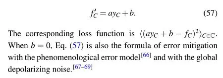
Alternatively, Czarniket al.[19]used the error-mitigation formula with two factoraandb:

8.1. The efficacy of Clifford learning

The efficacy of Clifford learning lies upon two results.This first result is that we can evaluate quantum-circuit error loss by sampling Clifford circuits[70]when the error model is independent of single-qubit gates. The underlying reason is that Clifford circuits formulate a unitary-2 design,[71]hence we have where U is the set of circuits when single-qubit gates are arbitrary unitary. When the error model depends on single-qubit gates,Eq.(58)does not hold in general. However we can still obtain a reliable estimation of the loss over unitary circuits using the method of hybrid sampling,[70]where a few gates in the circuit can be general unitaries while the other gates are all Clifford.

The second result is that,the bias can be complete eliminated in the ideal case such as when learning-based PEC finds the optimal quasi-probabilities.[18]Even for simple formulas such as that in Eq.(57),the bias is sufficiently reduced.[66,72]The results in Ref.[66]suggest that, iff＇Cis optimized using Clifford circuits,it holds that

whereNis the number of gates.

Sampling Clifford circuits is efficient if we use the importance Clifford sampling technique.[66]Suppose that the observable is a Pauli operator, the error-free result of a Clifford circuit is either 0 or±1. These Clifford circuits whose error-free results are zero do not contribute to the loss in Eq. (56), because their erroneous results are also zero when subjected to Pauli errors. For example,ρefis an error-free final state of a Clifford circuit with Tr(Oρef)=0. When subjected to a depolarizing channel, the erroneous final state isρ=(1-α)ρef+αI,whereαis the depolarizing rate,whose expected output is also zero. Importance Clifford sampling efficiently produces Clifford circuits with±1 outcomes,thus the loss can be efficiently estimated.

9. Combined methods

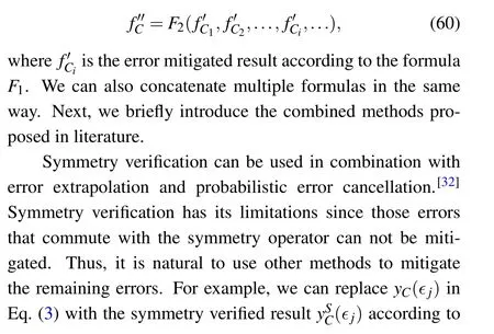
Multiple error mitigation methods can be used in combination when quantum computing with one method individually can not achieve a satisfactory accuracy. We can in principle take the output of one error-mitigated method as the input of another. For any two error mitigation formulasF1andF2,the concatenated formula is

Probabilistic error cancellation and error extrapolation can also be used in combination.[32,73]We can use error extrapolation to determine the gate-wise decomposition in Eq. (20) for noise-agnostic gates, i.e., we can replaceUi,βiwith the error-boosted gateUi(∊βi) and determine the quasiprobabilitiesλi,βiusing the error extrapolation method. On the other hand,if we have the tomographic knowledge on the noise operations, we can use PEC to effectively decrease the noise rate.We can use the results at several different decreased noise rates as the data points in error extrapolation. For example, in Eq. (3),∊jcan be considered as thej-th error rate reduced using PEC.

The framework of generalized subspace expansion[74]enables us to take the outputs of error extrapolation and virtual distillation as the inputs of subspace expansion. The general framework permits us to write the entries ofAin Eq. (47) asAi j=Tr(ρ(i)ρ(j)H).We can letρ(i)be either the output of virtual distillation withicopies,or the output ofi-th error-boosted quantum circuit.

All kinds of methods can be used in combination with Clifford-circuit learning.[66,75]For example, given a twopoints error extrapolation formula

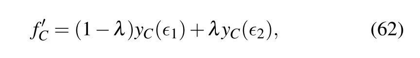
we can use the Clifford-circuit learning method to determine the parameterλ. Another example is,we can always take the error mitigated result as the input of Clifford circuit learning.Supposing thatf＇Cis the error-mitigated result via PEC or virtual distillation,we can further improve the result byf＇＇C=a f＇C,whereais determined using Clifford-circuit learning.

10. Summary

In this paper,we provide a thorough overview of the stateof-the-art QEM methods in a general form,where each method is expressed as an error mitigation formula. With the formula,we can concatenate any two or more QEM methods by replacing the inputyto the high-level method with outputf＇of the low-level method. The formula can be further optimized with lower bias and variance using the Clifford-circuit learning method, where the formula is written as a parameterized function.

Note that the qubit cost and implementation complexity are not reflected in the error mitigation formula.The efficiency of some methods,for instances PEC and Clifford circuit sampling, is maximized under the assumption of sampling random circuits. Random circuit sampling is necessary in Pauli twirling to convert general errors into Pauli errors,which have favorable properties in QEM.In this regard,some QEM methods are easier to implement. For example, as error extrapolation requires no random circuit sampling, it can be implemented with only a few circuits.

The bias and the variance of the QEM estimator depend on the error mitigation formula and estimator of eachyC. In general, there is room to optimizeyCestimators to maximize the performance of QEM. For example, in PEC, circuit executions are allocated according to importance sampling. With the QEM formula, we can analyze the bias and the variance using the standard approach,e.g.,propagation of uncertainty.

Error mitigation methods are important for quantum computing on NISQ devices. Compared with QEC, QEM can work in quantum circuits with high error rates. On the other hand, as the variance increases with the circuit size, more sampling and circuit executions are required to reduce the variance, thus QEM is not as scalable as QEC. However, as the QEM technique continuously evolves,we anticipate some benchmarking tools to be developed to reduce the circuit execution overhead. Meanwhile, QEM could be used in part of QEC to reduce the qubit cost when fault-tolerant technology becomes available.[76-79]

Acknowledgments

This work is supported by the National Natural Science Foundation of China (Grant Nos. 11875050 and 12088101)and NSAF(Grant No.U1930403).