Variational quantum support vector machine based on Hadamard test

Li Xu,Xiao-Yu Zhang,Jin-Min Liang,Jing Wang,Ming Li,Ling Jian and Shu-qian Shen

1 College of Science,China University of Petroleum,Qingdao 266580,China

2 School of Mathematical Sciences,Capital Normal University,Beijing 100048,China

3 School of Economics and Management,China University of Petroleum,Qingdao 266580,China

Abstract Classical machine learning algorithms seem to be totally incapable of processing tremendous amounts of data,while quantum machine learning algorithms could deal with big data with ease and provide exponential acceleration over classical counterparts.Meanwhile,variational quantum algorithms are widely proposed to solve relevant computational problems on noisy,intermediate-scale quantum devices.In this paper,we apply variational quantum algorithms to quantum support vector machines and demonstrate a proof-of-principle numerical experiment of this algorithm.In addition,in the classification stage,fewer qubits,shorter circuit depth,and simpler measurement requirements show its superiority over the former algorithms.

Keywords:quantum support vector machine,Hadamard test,variational quantum algorithm

1.Introduction

Machine learning[1]is a multi-field interdisciplinary subject,which is based on studying how computers simulate or realize human learning behavior to acquire new knowledge or skills,then reorganize the existing knowledge structure and improve its performance.There are two types of machine learning,supervised learning and unsupervised learning,the difference is whether the label is stamped in advance.A support vector machine(SVM)[1,2]for classification is a frequently-used supervised learning algorithm.Like all machine learning algorithms,SVM is weak in facing billions and trillions of training data.Due to the exponential acceleration of quantum algorithms over classical algorithms[3,4],a quantum support vector machine(QSVM)[5]emerges as the times require,and the experiment also proves its feasibility[6].In the last decade,research and application of SVM has always been a hot topic,such as least squares SVM(LS-SVM)[7,8],multiclass SVM[9–11],quantum multi-class SVM[12,13],and twin support vector machine[14–16]etc.

In recent years,many classical algorithms that can replace quantum algorithms have been proposed,and they also achieve the exponential acceleration that quantum algorithms can achieve.Due to Tang’s[17]query and challenge to quantum machine learning,many quantized versions of classical machine learning are eclipsed.Since quantum random access memory[18,19]may be replaced by‘sample and query access’and quantum machine learning algorithm is not accelerated in the process,hitting a number of scholars who study how to quantize classical algorithms.Before the advent of quantum computers,we could not get an accurate result from this debate.At this time,the practicability of the variational quantum algorithm shows its value.Up to now,variational quantum algorithms have been widely used and solved some problems that are beyond the power of classical computers[20–24].

The manuscript is organized as follows.We first review the SVM and QSVM algorithms and give the quantum circuit diagrams.We then propose a variational QSVM algorithm that uses the most fundamental measurement method—Hadamard Test—to complete the classification stage.Finally,the numerical experiment shows the feasibility of the algorithm.

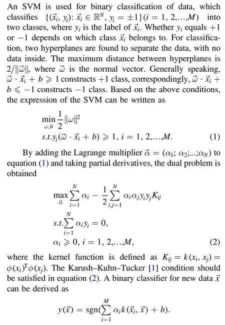
2.Support vector machine

3.Quantum least squares support vector machine

In this section,we give a short review of[5,6].Suppose there are oracles that encode training data to quantum states

The core idea is the least square method,which transforms the quadratic process into solving linear equations.The introduction of slack variables replaces the inequality constraint with the equality constraint

The slack variableseirepresent the degree to which the sample does not satisfy the constraint,where user-specified γ determines the relative weight of the training error and the SVM objective.The following equation can be obtained by calculating the partial derivative of the dual Lagrange problem

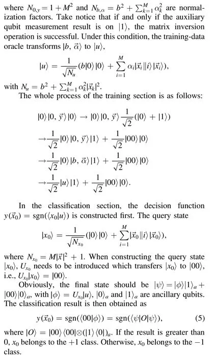
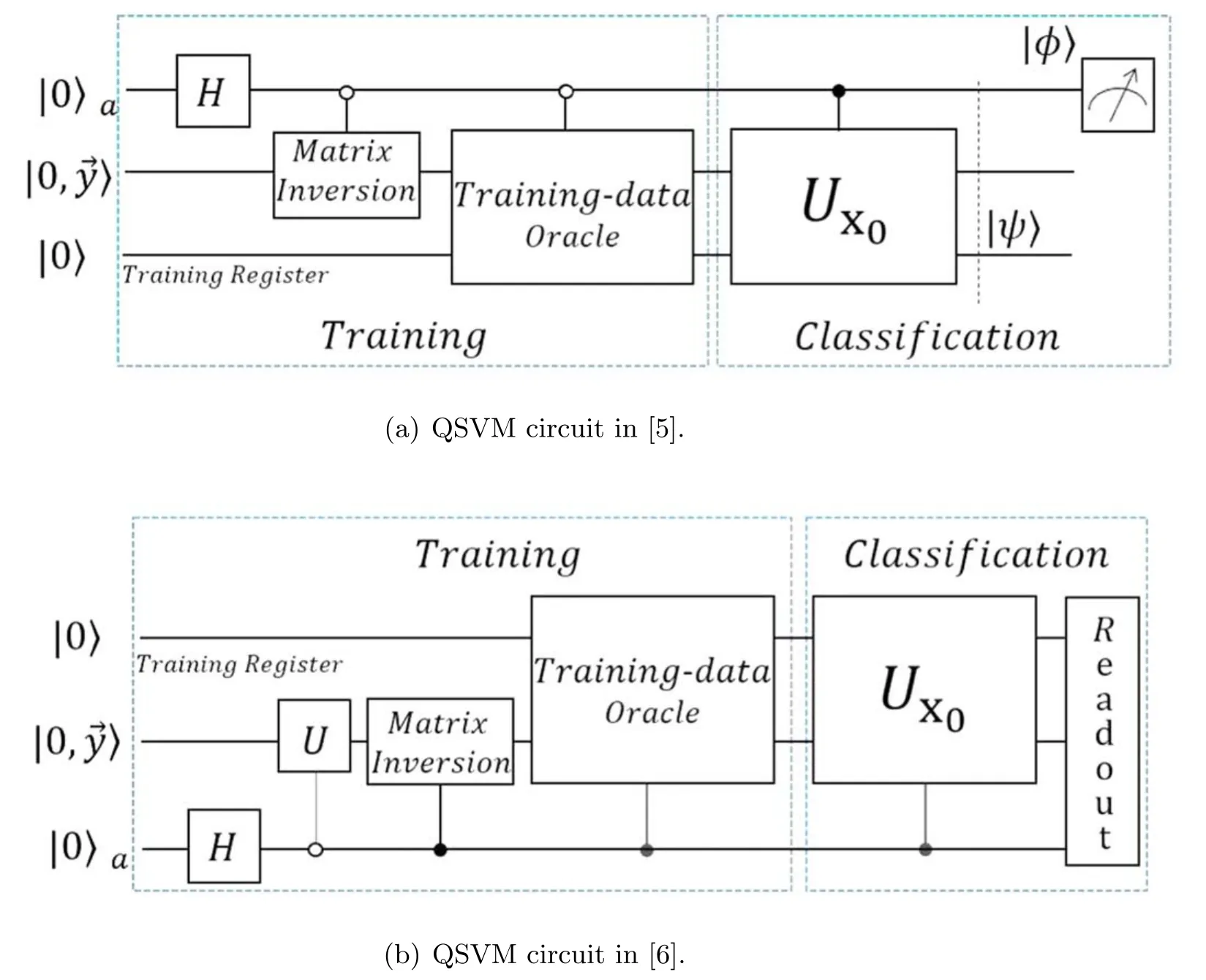
Figure 1.Brief circuit diagram of QSVM.The Matrix Inverse is employed to acquire the hyperplane parameters.The Training-data Oracle prepares|u〉.The information of the query state is stored in Ux0.The auxiliary qubit used to solve the equation is omitted.(a).The QSVM algorithm in this section is based on(b).

4.Variational quantum support vector machine

In this section,we propose a variational QSVM algorithm that divides training and classification into two parts and perform a numerical simulation to verify the practicability.

4.1.Training part

The matrixFin(4)can be decomposed in the form of

where

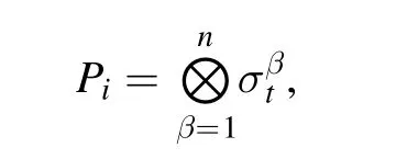
t=0,x,y,z,that is,σtis the Pauli matrix.In order to get each δi,we need to use the following formula

Thus,we have

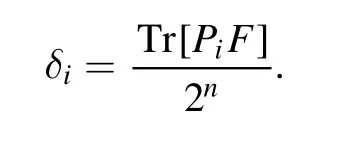
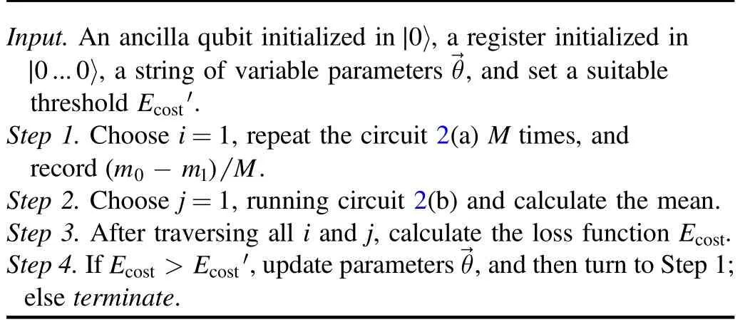
Of course,applying Pauli decomposition to the kernel function of a QSVM is the simplest,but it may be inefficient.Thus,we will try to find some more effective decomposition methods[26–28]to improve the feasibility of the algorithm.After the decomposition of equation(6)is finished,the next step is training the QSVM,and the circuit is shown in figure 2(a).Due to our choice of the Hadamard test measurement method,the loss function can be defined as follows

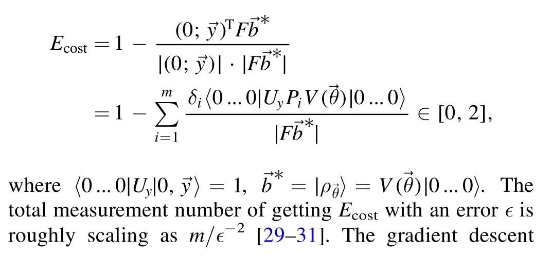
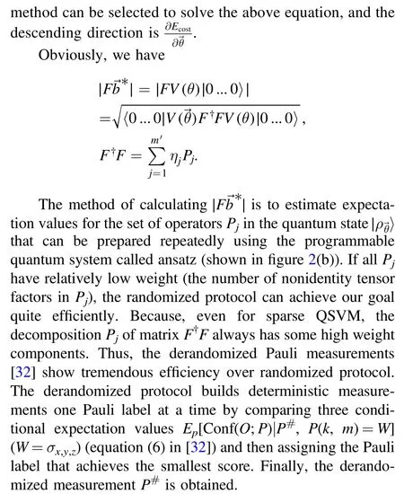
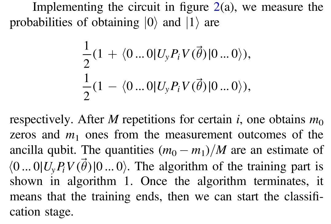
Figure 2.Brief circuit diagrams of training part of variational QSVM.(a)Calculating the molecular part of the loss function.can be expressed as a product of L unitaries Vl(θl)sequentially acting on the input state|0...0〉.As indicated,each unitary Vl(θl)can in turn be decomposed into a sequence of parametrized and unp→arametrized gates.Uy is a unitary matrix that satisfiesCalculating the denominator of the loss function.Theθ is consistent with(a),Pj is the Pauli decomposition of F†F.Efficient derandomization Pauli measurements are employed at the end of the circuit,rather than random single-qubit measurements.

4.2.Classification part

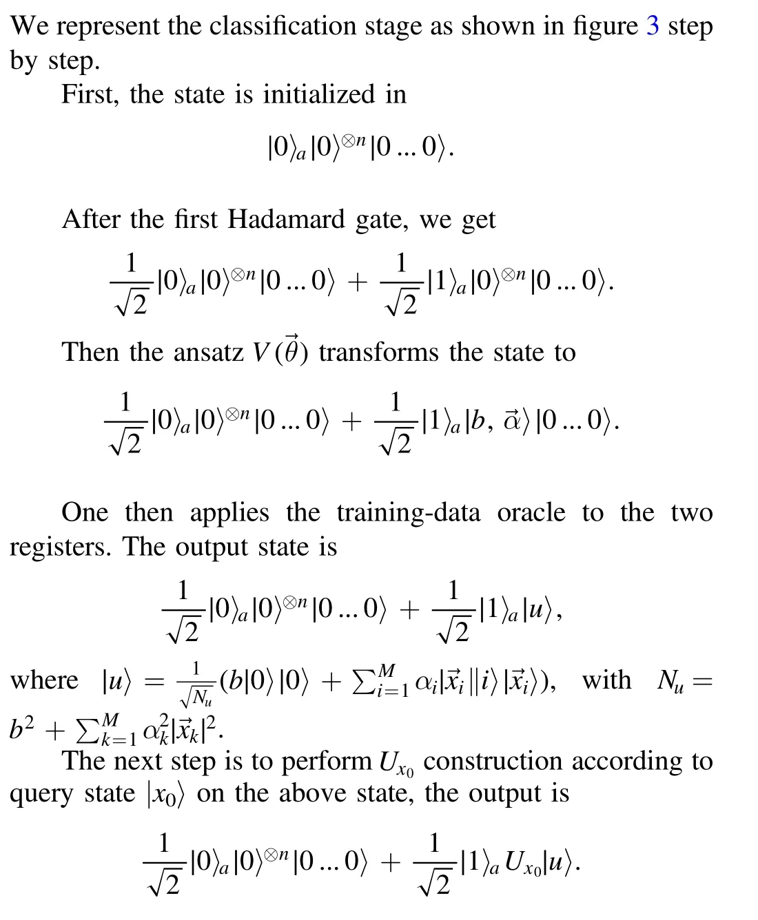
After the last Hadamard gate operating in the above state,we have the terminal state

Finally,the probabilities of measuring|0〉and|1〉are

respectively.Similarly,we can repeat this lineTtimes and gett0zeros andt1ones.Ift0>t1,the classification result will be positive;otherwise,it will be negative.At this point,the algorithm ends.

In the classification stage,we do not need to calculate the exact value of〈x0|u〉,we just need to know whether it is positive or negative.In other words,we just need to compare the size oft0andt1.As mentioned above,estimating the value of〈x0|u〉with an error ∊demands measurements ∊−2times

The fault tolerance classification result will be revealed by

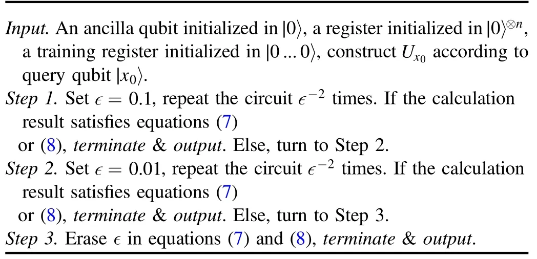
In order to improve the classification efficiency,we set two thresholds ∊=0.1,0.01,and the detailed process of the algorithm is shown in algorithm 2.

Algorithm 1.Training variational QSVM

Algorithm 2.Classification variational QSVM

4.3.Numerical experiment simulation

In order to certificate the feasibility of the algorithm and its advantageous aspects over the conventional QSVM,we devise numerical experiments to test and verify it.For convenience,we quote the experimental data of[6].Besides,to keep consistent with this,we discard the offset termband take.According to the data in figure 4(a),one educes

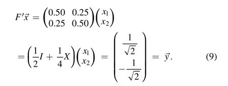
Figure 3.Brief circuit diagram of classification part of variational QSVM.The is the one in the last cycle of algorithm 1.The Training-data Oracle prepares state|u〉.Ux0 contains the information of query state.

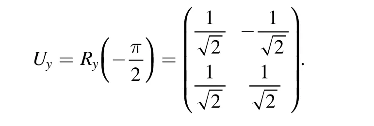
The unitary matrixUyin figure 2(a)encodingcan be written as

To get the mean of∣F′b∣*,we have

The correspondingly derandomized Pauli measurements areZandX.Here,the PauliZmeasurement could substitute for PauliXmeasurements by adding a Hadamard gate to the final states.In addition,the gradient of θ is

After all the preparations are ready,we conduct numerical simulation,and the iterative line chart is shown in figure 4(b).Then we construct the classification circuit shown in figure 5,where the hardware efficient ansatz with θ=−1.57 will be the subsequent classification operation as a subroutine.

We implement this task on today’s current state-of-the-art quantum computer using the IBM quantum experience platform where the experimental circuit diagram and experimental results are shown in figures A1 and A2 in the appendix.For comparison,but due to the limitation of qubits,we only give the experimental circuit diagram of applying the HHL algorithm to the QSVM(shown in appendix figure A3).The results of classification results are shown in table 1.It can be seen that by adding the fault-tolerant classification formula,we can predict the results 100% accurately when we measure only 100 times.

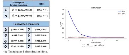
Figure 4.(a)Experimental data of[6],where the feature values are chosen as the vertical ratio and the horizontal ratio.The training data is in a standard font(Times New Roman).The arbitrary chosen handwritten samples for classification and their feature vectors.(b)Loss function image optimized by gradient descent penalty.The calculation result is simulated by Python.

Figure 5.The classification circuit.The rotation angles .The last two controlled Ry(θi)gates form Ux0,with.

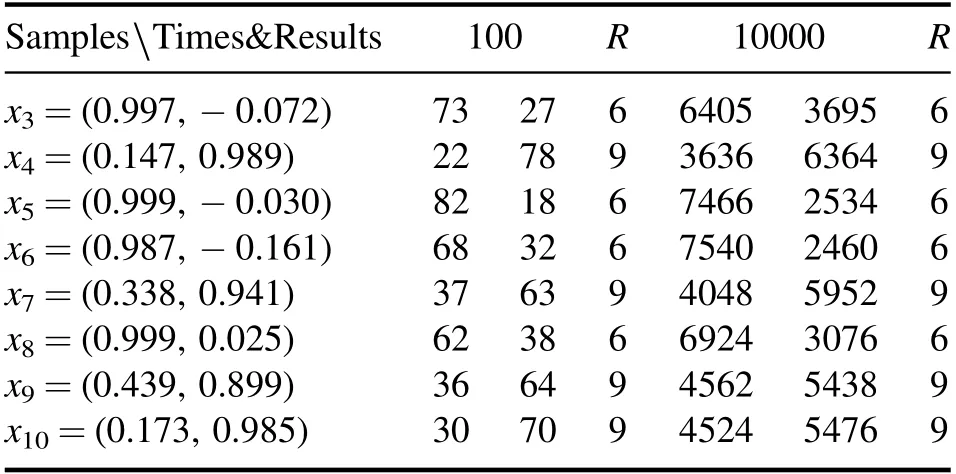
Table 1.The classification results of samples.In the two columns below the number of measurements,the left one is the number of times the auxiliary qubit measures 0 and the right is obtaining 1.

4.4.Advantage analysis

The QSVMs shown in figure 1 have put training and classification in a circuit which means that they run the whole route every time one classifies a new data.Once the classification data is much larger than the training data,the algorithms will lead to a lot of redundant operations.In practice,the long line of figure 1(a)and the complex measurement mode of figure 1(b)will be an obstacle to the successful implementation of the algorithm.Since the variational QSVM divides training and classification into two parts,when the training stage is completed,and it will turn to the classification circuit.When classifying,our algorithm only requires Hadamard test measurements and owns a shorter line depth,which is more amenable to execution on near-term devices.

Here,we analyze the circuit depth and qubits numbers of our algorithm compared with the algorithm in[5].Our algorithm needs 2,1 and 3 qubits,respectively,in solving equations part,calculating modules part and classifying parts.In contrast,if one adopts the HHL algorithm directly to the QSVM,there must be 4 qubits—1 ancilla qubit(abbreviateda1),2 register qubits,and 1 qubit storing the input message and output result—in the stage of solving equations.Meanwhile,in constructing the statethere must be 1 more ancilla qubit(abbreviateda2)and 1 register qubit for building|u〉according to the output of the HHL algorithm.The total qubits number of applying the HHL algorithm to the QSVM is 6.

When applying the HHL algorithm to equation(9),we have to use 2 qubits for the register,despite the fact that the more registered qubits the more accurate result,and the fewer registered qubits the easier the quantum circuit.In the phase estimation stage,if we only use 1 registered qubit,the estimated eigenvalue ofF′is either 0 orwhich leads to a great error.Although 3 registered qubits could estimate the eigenvalue among,i=0,1,…,7,it will bring a great burden on the construction of quantum circuits.Besides,the addition ofa2produces a number ofC2(U)gates which can be decomposed into 5 universal quantum gates.Thus,the circuit is much deeper than the variational QSVM circuit.Furthermore,the quantum circuit is implemented successfully under the circumstancesa1measures 1 which means that the run times exceed the variational QSVM circuit.

In a more general sense,suppose the dimension ofF′ isN×N,one applies the HHL algorithm to the QSVM demands at least 3 +3 logNqubits overall.The corresponding part of the variational QSVM needs1 +logN,logNand 1 +2 logNqubits,gathered 2 +4 logN.It can be seen that with the increase ofN,the number of qubits required by applying the HHL algorithm to the QSVM is less than that of the variational QSVM.However,the number of qubits used in the phase estimation stage 1 +logNis only the minimum number we assume,and the accuracy cannot be guaranteed.Meanwhile,our algorithm shows great advantages in the depth of quantum circuits.

5.Conclusion and outlook

We propose a quantum–classical variational algorithm to solve the QSVM based on the Hadamard test and construct a loss function that is only suitable for vectors’ own equal module length.That is,it applies to quantum states.Besides,our algorithm adopts the derandomization Pauli measurements protocol which shows strong advantages over random Pauli measurements due to the high weight decomposition.We have carried out simulated quantum experiments to prove the feasibility of the algorithm.In the future,we will also consider applying this algorithm to a multi-classification QSVM.

Acknowledgments

This work is supported by the Shandong Provincial Natural Science Foundation for Quantum Science No.ZR2020LLZ003,ZR2021LLZ002.

Appendix

As shown in figures A1,A2 and A3,it is obvious that the variational QSVM is much more efficient in classification.

Figure A1.The experimental classification circuit of variational QSVM.

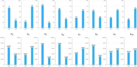
Figure A2.Experimental data.

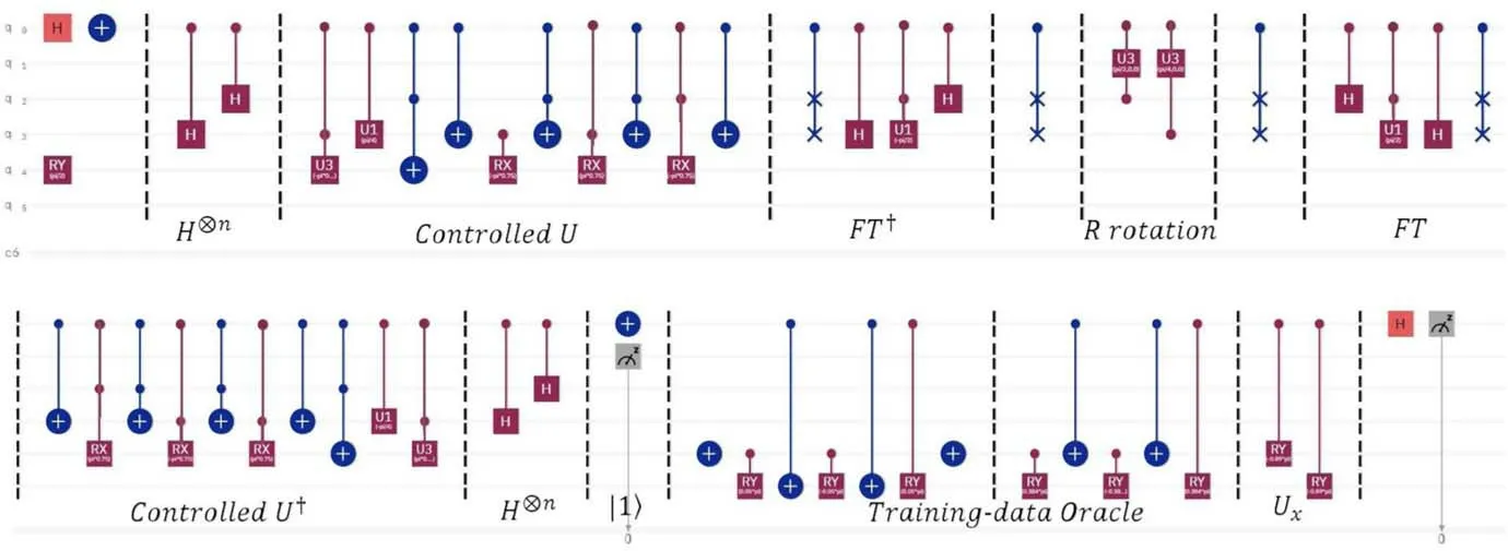
Figure A3.The experimental circuit of applying the HHL algorithm to the QSVM.Here,q0 refers to the ancilla a2,q1 refers to the ancilla a1,q2 and q3 are registers,q4 stores the input and output message,and q5 is the training register.Besides,the C2(U)gates in the stage of the HHL algorithm should be decomposed into universal quantum gates.

ORCID iDs