Classifying Galaxy Morphologies with Few-shot Learning

Zhirui Zhang ,Zhiqiang Zou ,Nan Li ,and Yanli Chen

1 College of Computer,Nanjing University of Posts and Telecommunications,Nanjing 210023,China

2 Jiangsu Key Laboratory of Big Data Security and Intelligent Processing,Nanjing 210023,China

3 Key Laboratory of Optical Astronomy,National Astronomical Observatories,Chinese Academy of Sciences,Beijing 100101,China;nan.li@nao.cas.cn

4 University of Chinese Academy of Sciences,Beijing 100049,China

Abstract The taxonomy of galaxy morphology is critical in astrophysics as the morphological properties are powerful tracers of galaxy evolution.With the upcoming Large-scale Imaging Surveys,billions of galaxy images challenge astronomers to accomplish the classification task by applying traditional methods or human inspection.Consequently,machine learning,in particular supervised deep learning,has been widely employed to classify galaxy morphologies recently due to its exceptional automation,efficiency,and accuracy.However,supervised deep learning requires extensive training sets,which causes considerable workloads;also,the results are strongly dependent on the characteristics of training sets,which leads to biased outcomes potentially.In this study,we attempt Few-shot Learning to bypass the two issues.Our research adopts the data set from the Galaxy Zoo Challenge Project on Kaggle,and we divide it into five categories according to the corresponding truth table.By classifying the above data set utilizing few-shot learning based on Siamese Networks and supervised deep learning based on AlexNet,VGG_16,and ResNet_50 trained with different volumes of training sets separately,we find that few-shot learning achieves the highest accuracy in most cases,and the most significant improvement is 21% compared to AlexNet when the training sets contain 1000 images.In addition,to guarantee the accuracy is no less than 90%,few-shot learning needs～6300 images for training,while ResNet_50 requires～13,000 images.Considering the advantages stated above,foreseeably,few-shot learning is suitable for the taxonomy of galaxy morphology and even for identifying rare astrophysical objects,despite limited training sets consisting of observational data only.

Key words:Galaxies– Galaxy:morphological classification– Method:neural networks

1.Introduction

Galaxy morphology is considered a powerful tracer to infer the formation history and evolution of galaxies,and it is correlated with many physical properties of galaxies,such as stellar populations,mass distribution,and dynamics.Hubble invented a morphological classification scheme for galaxies(Hubble 1926) and pioneeringly revealed the correlation between galaxy evolutionary stages and their appearance in optical bands.Hubble sequence principally includes early-type galaxies (ETGs) and late-type galaxies (LTGs);ETGs mostly contain older stellar populations and have few spiral structures,while LTGs hold younger stellar populations and usually present spiral arms-like features.The above correlation has been studied widely and deeply in the past decades with increasing observational data of galaxies.Predictably,relevant investigations will be significantly advanced with enormous data from the upcoming large-scale imaging surveys,such as LSST,6https://www.lsst.orgEuclid7https://www.euclid-ec.org/and CSST.8http://www.bao.ac.cn/csst/

Galaxy morphology classification is started with visual assessment (de Vaucouleurs 1959,1964;Sandage 1961;Fukugita et al.2007;Nair &Abraham 2010;Baillard et al.2011) and has lasted for decades as the mainstream approach in the field.In the 21st century,the volume and complexity of astronomical imaging data have increased significantly with the capability of the new observational instruments,such as the Sloan Digital Sky Survey9https://www.sdss.org/(SDSS) and the Hubble Space Telescopes10https://hubblesite.org/(HST).To make the classification more efficient and accurate,astronomers developed non-parametric methods to extract morphological features of galaxies,such as the concentration-asymmetry-smoothness/clumpiness (CAS) system,the Gini coefficient,and the M20 parameter (Abraham et al.2003;Conselice 2003;Lotz et al.2004;Law et al.2007).Sets of evidence demonstrate the success of utilizing these approaches to represent galaxy morphologies,outperforming traditional human inspection because they eliminate subjective biases.However,encountering hundreds of millions or even billions of galaxy images from future surveys,the performance of the above CPU-based algorithms is inefficient.Hence,more effective techniques for Galaxy morphology classification in an automated manner,e.g.,machine learning,are necessary.

Machine learning algorithms have been widely used to classify galaxy morphology in the past years,for instance,Artificial Neural Network (Naim et al.1995),NN+local weighted regression (De la Calleja &Fuentes 2004),Random Forest (Gauci et al.2010),linear discriminant analysis (LDA,Ferrari et al.2015).Recently,deep learning has become more and more popular for classifying galaxy morphology (Lukic et al.2019;Zhu et al.2019;Cheng et al.2020;Gupta et al.2022) as its success has been proved adequately in industries,especially for pattern recognition,image description,and anomalies detection.Most cases for classifying galaxy morphologies are based on supervised deep learning due to its high efficiency and accuracy.Successful cases include generating the catalogs of galaxy morphologies for SDSS,the Dark Energy Survey11https://www.darkenergysurvey.org/(DES),and the Hyper Suprime-Cam12https://www.naoj.org/Projects/HSC/(HSC)Surveys(Dieleman et al.2015;Flaugher et al.2015;Aihara et al.2018).However,the results of supervised deep learning are strongly dependent on the volume and characteristics of the training set.First,requiring a large volume of data for training is determined by the complexity of the convolution neural networks,which typically comprise millions of trainable parameters.Hence,to make the training procedure converge correctly,one has to provide data points with a comparable amount to the number of parameters of the Convolutional Neural Network (CNN).Second,the best trained CNN model reflects the properties of the feature space covered by the training set.Thus,if the training set(simulated or selected by astronomers)is considerably biased from the real universe,supervised deep learning may consequently give biased results.Unsupervised learning has been adopted to avoid those disadvantages,but the corresponding classification accuracy is～10% worse than that of supervised manners (Cheng et al.2020,2021).

In this study,we attempt few-shot learning(Wang et al.2019)to classifying galaxy morphologies by proposing a model named SC-Net inspired by CNNs and the siamese network model (Chopra et al.2005).Concisely speaking,our method pairs images and compares the metrics between features of input images,which expands the sample size of the training set compared to feeding images directly into the CNN.Furthermore,the region of feature space covered by the training set can be enlarged more effectively by involving rare objects and pairing them with other objects.Thus,in principle,SC-Net model simultaneously improves the two drawbacks of traditional supervised deep learning.To quantify the improvements,we designed an experiment with adopting galaxy images from the Galaxy Zoo Data Challenge Project on Kaggle13https://www.kaggle.com/c/galaxy-zoo-the-galaxy-challengebased on Galaxy Zoo 2 Project (Willett et al.2013),then compared the classification results to those with AlexNet (Krizhevsky et al.2012),VGG_16 (Simonyan &Zisserman 2014),and ResNet_50 (He et al.2015).The outcomes show that our method achieves the highest accuracy in most cases and requests the most miniature training set to satisfy a given accuracy threshold (see Section 5 for more details).Therefore,foreseeably,SC-Net model is suitable for classifying galaxy morphology and even for identifying rare astrophysical objects in the upcoming gigantic astronomical data sets.The code and data set used in this study are publicly available online.14https://github.com/JavaBirda/Galaxy-Morphologies-

The paper is organized as follows:Section 2 introduces the data sets and data enhancement.Deep learning models,including CNNs and siamese Network,are described in Section 3.Section 4 presents the experimental process of this study.Results of this work are analyzed and summarized in Section 5.Finally,we draw discussion and conclusions in Section 6.

2.Data Sets

The SDSS captured around one million galaxy images.To classify the galaxy morphology,the Galaxy Zoo Project was launched (Lintott et al.2008),which is a crowd-sourced astronomy project inviting people to assist in the morphological classification of large numbers of galaxies.The data set we adopted is one of the legacies of the Galaxy Zoo Project,and it is publicly available online for the Galaxy-zoo Data Challenge Project.

The data set provides 28,793 galaxy morphology images with middle filters available in SDSS (g,r,and i) and a truth table including 37 parameters for describing the morphology of each galaxy.The 37 parameters are between 0 and 1 to represent the probability distribution of galaxy morphology in 11 tasks and 37 responses(Willett et al.2013).Higher response values indicate that more people recognize the corresponding features in the images of given galaxies.The catalog is further debiased to match a more consistent question tree of galaxy morphology classification (Hart et al.2016).

To simply the classification problem,we reorganize 28,793 images into five categories:completely round smooth,inbetween smooth,cigar-shaped smooth,edge-on,and spiral,according to the 37 parameters in the truth table.The filtering method refers to the threshold discrimination criteria in Zhu et al.(2019).For instance,when selecting the completely round smooth,values are chosen as follows:fsmoothmore than 0.469,fcomplete,roundmore than 0.50,as shown in Table 1.

We then build six training sets with different numbers of images to test the dependence of the performance ofclassification algorithms on the volume of training sets,details of the training sets are shown in Table 2.In Section 4,we will train all the deep learning models with 28,793,20,000,15,000,10,000,5000,and 1000 images,respectively,and compare their performances thoroughly.

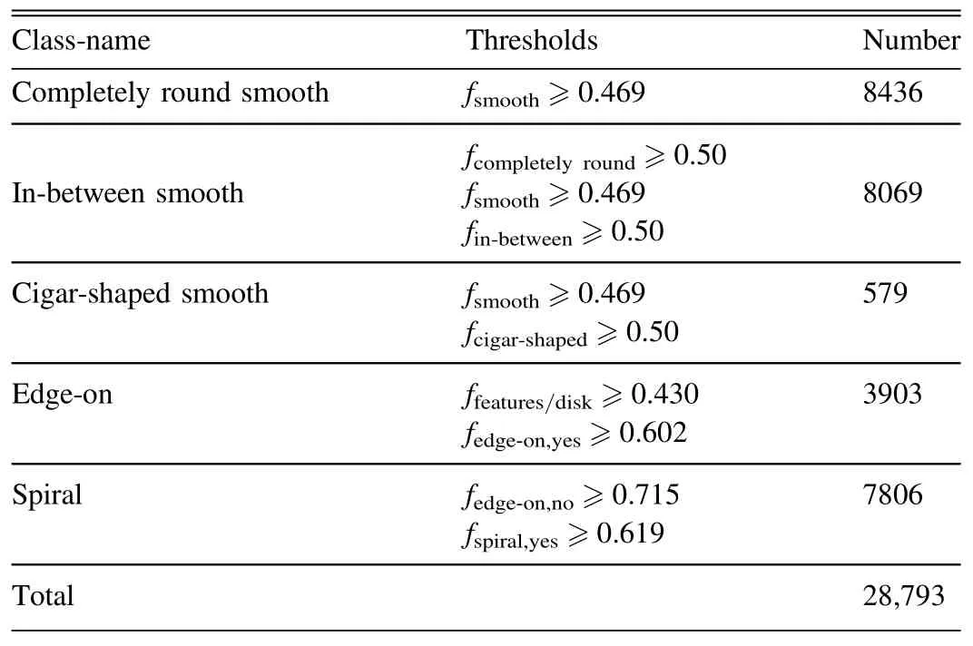
Table 1 The Classification of 28,793 Samples

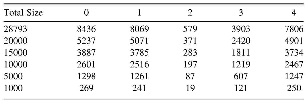
Table 2 The Amount of Data in Each Category Under Different Data Sizes

3.Methodology

The few-shot learning proposed in this study is based on a model named SC-Net,including a CNN and a siamese network.We use CNNs to extract features,and then train the model according to the idea of the siamese network for classifying galaxy morphologies.Explicitly,the CNNs section introduces the feature extraction process and several traditional CNNs(LeCun et al.1998;Krizhevsky et al.2012;Simonyan&Zisserman 2014;He et al.2015) for classification;the siamese network section describes the few-shot learning method and the structure of the siamese network.

3.1.Convolution Neural Networks

CNN is a feed forward neural networks which includes convolutional computation and deep structure,and is one of the representative algorithms of deep learning.CNN is essentially input-to-output mappings that learn mapping relationships between inputs and outputs without requiring any precise mathematical expressions so that CNN has been widely used in the field of computer vision in recent years.

The schematic of image feature extraction with CNN mainly consists of the following three main layers:convolution layer,pooling layer and fully connected layer.The convolution layer for feature extraction of the image is built by dot multiplication operation of the image and convolution kernel.Each pixel ofthe image and the weight of the convolutional kernel are computed through convolution layer and the calculation process is shown in Equation (1)

where the f function is an activation function.We usually use Rectified Linear Units (Relu) (Glorot et al.2011) as the activation function defined in Equation (2).wm,nmeans the weight,xi+m,j+nmeans input data of current layer,wbrepresents bias,and ai,jdescribes the output data of current layer.

Relu turns a negative value into zero.The image size obtained by the convolution operation is related to certain factors,such as the size of the convolution kernel,the convolution step size,the expansion method and the image size before convolution.The formula description of convolution operation is shown in Equation (3)

where W1means the width of input data,H1means the height of input data,F represents the size of convolution kernels,P describes the padding size and S means stride,W2and H2denote the value of W1and H1after being calculated.The pooling layer is applied to reduce the image size while retaining important information.Max-pooling retains the maximum value of feature map as the resulting pixel value,while average-pooling retains the average value of feature map as the resulting pixel value.The fully connected layer acts as a“classifier” for the entire CNN after convolution,activation function,pooling and other deep networks.The classifying results are identified by the fully connected layer.

In the past 20 yr,traditional CNN algorithms for image classification have made breakthroughs (LeCun et al.1998).AlexNet for ImageNet competition was proposed by Hinton’s student Alex Krizhevsky (Krizhevsky et al.2012),which established the status of CNNs in computer vision.VGGNet(Simonyan &Zisserman 2014) was proposed by the Oxford University Computer Vision Group in 2014,which has good generalization ability and can be easily migrated to other image recognition projects.Kaiming He et al.proposed the ResNet(He et al.2015)in 2015,which solves the problem of gradient explosion due to depth of model layers.

Although the development of deep learning has made great achievements,deep learning models are strongly dependent on the size and quality of the data set.Traditional deep learning models cannot get a better result when lacking plenty of samples.To solve this problem,some researchers introduced data augmentation methods and generate simulated samples,such as GAN (Goodfellow et al.2014),which alleviates the difficulty of insufficient samples to a certain extent.However,its result is not very ideal because of the deviation between the real world data and simulated samples.Therefore,a new method is needed to solve this problem.

3.2.Siamese Network

To solve the problem of lacking of enormous samples with high quality mentioned in Section 3.1,this study introduces the few-shot learning (Wang et al.2019).Few-shot learning is an application of Meta Learning (Schweighofer &Doya 2003) in the field of supervised learning,which is mainly used to solve the problem of model training with a small number of classified samples.Few-shot learning is divided into three categories:model-based method,optimization-based method (Wang et al.2019) and metric-based method.

The model-based methods aim to learn the parameters quickly over a small number of samples through the design of model structure,and directly establish the mapping function between the input value and the predicted value,such as memory-enhancing neural network (Santoro et al.2016),meta networks (Munkhdalai &Yu 2017).The optimization-based methods consider that ordinary gradient descents are inappropriate under few-shot scenarios,so they optimize learning strategies to complete the task of small sample classification,such as LSTM-based meta-learner model (Ravi &Larochelle 2016).The metric-based methods measure the distance between samples in the batch set and samples in the support set by using the idea of the nearest neighbor,such as the siamese network (Koch et al.2015).Considering the universality and conciseness of metric distance,this study chooses the metric-based method.

The siamese network is a metric-based model in few-shot learning,which was first proposed in 2005(Chopra et al.2005)for face recognition.The basic idea of the siamese network is to map the original image to a low-dimensional space,and then get feature vectors.The distance between the feature vectors is calculated through the Euclidean distance.In our study,the distance between the feature vectors from the same galaxy morphology should be as small as possible,while the distance between the feature vectors from the different galaxy morphology should be as large as possible.The framework of the siamese network is shown in Figure 1 (Chopra et al.2005).

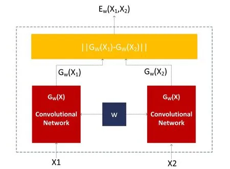
Figure 1.Siamese Architecture.The left and right input different data,and calculate the similarity between them after feature extraction.

In the siamese network,the structures of two networks on the left and right share the same weights (W).The input data,denoting(X1,X2,Y),are two galaxy morphology and the label that measures the difference between them.The label Y will be set to 0 when X1and X2belong to the same galaxy morphology,and it will be set to 1 when X1and X2belong to different galaxy morphology.The feature vectors Gw(X1)and Gw(X2) of low-dimensional space are generated by mapping X1and X2,and then their similarity is computed by Equation (5)

The SC-Net makes Ew(X1,X2) as small as possible when Y=0 and makes Ew(X1,X2) as large as possible when Y=1.Contrastive Loss(Hadsell et al.2006) is selected in SC-Net as the loss function,which makes the originally similar samples are still similar after dimensionality reduction and the original dissimilar samples are still dissimilar after dimensionality reduction.The formula for the contrast loss function is shown in Equation (6)

When the input images belong to the same galaxy morphology,the final loss function depends only on LG(EW),and when the input images belong to different galaxy morphology,the final loss function depends on LI(EW).LG(EW) and LI(EW) are defined in Equations (7) and (8).The constant Q is set to the upper bound of EW

As so far,we can train the SC-Net model according to the architecture and loss function as described above.Then the classified results will be obtained.The advantage of this method is to fade the labels,making the network have good extension.Moreover,this approach increases the size of the data set by pairing data operation,so that deep learning network will achieve better effect with the small amount of data.For the above reasons,we adopt the siamese network and put forward the SC-Net model.

4.Experiments

The workflow of our SC-Net model is shown in Figure 2.The whole procedure includes four stages:the first stage is to preprocess data with the method introduced in Section 4.1;the second stage is to generate the training set via re-sampling or sub-sampling the preprocessed data;the third stage is to train model based on the networks described in Section 4.2;the last stage is to classify the images using the trained model.Section 4.3 describes the details of the implementation of these experiments.

4.1.Data Pre-processing

The experiment data sets consist of 28,793 images with 424×424×3 pixels in size.The training time is sensitive to the size of images,and the features of galaxies are primarily concentrated at the centers of the original images.Therefore,we crop and scale the original images first,then arrange them to training sets.The workflow of data preprocessing is shown in Figure 3,which is the same as shown by Zhu et al.(2019).We first crop the original images from 424×424 pixels to 170×170 pixels,considering the image centers as origins.Then,the images with 170×170 pixels are resized to 80×80 pixels.Finally,we repeat the first step to crop the images with 80×80 pixels to 64×64 pixels.

As is mentioned in Section 2,we have divided the 28,793 images into five categories according to the truth table with the approach used in Zhu et al.(2019) and organized six data sets to implement comparative experiments for quantifying the advantages of the SC-Net over traditional CNNs.The six data sets contain 1000,5000,10,000,15,000,20,000,and 28,793 images.The preprocessed data sets have the same organization but images with 64×64×3 pixels,and examples from each category are shown in Figure 4.

The data form that the SC-Net model takes is (X1,X2,Y),where X1and X2represent a pair of images,and Y is the label of the correlation between X1and X2.For example,X1is in category edge-on,and X2is selected in the same category,then Y was set to 0.To balance positives and negatives in training sets,every time we create a positive data point,we create a negative data point by randomly selecting an image from other categories.

4.2.Deep Learning Models

For comparison,we first build three approaches based on traditional CNNs:(1) AlexNet (Krizhevsky et al.2012),(2)VGG_16 (Simonyan &Zisserman 2014),and (3) ResNet_50(He et al.2015).(1) AlexNet consists of five convolutional layers and three fully connected layers.The network structure is successively conv11-96,max pool,conv5-256,maxpool,conv3-384,conv3-384,conv3-256,maxpool.(2)The network structure of VGG_16 is constructed by modularization.The first and second modules are divided into two convolutional layers and a max-pooling layer,and the last three modules are composed of three convolutional layers and a max-pooling layer.The number of channels in the convolutional kernel increases from 64 to 512,and finally,three fully connected layers are added,with the number of neurons being 4096,4096,and 1000 successively.There are 13 convolution layers and three full connection layers in total.(3)Resnet_50 consists of a convolutional layer,16 residual modules,and a full connection layer.The residual module has an identity block and a convolutional block composed of three convolutional layers and a shortcut.The difference lies in that the identity block ensures the consistency of input and output data.The input images of all CNN models are of 64×64 pixels in three channels,and the outputs are vectors of 1×5.The remaining parameters,such as the network hierarchy and hyperparameters,were referred to in the original papers.

The architecture of SC-Net is shown in Figure 5,which consists of two parts.The first part is for extracting features with a CNN,and the second part calculates the similarity between the feature vectors obtained from the first part.The outputs of the SC-Net are the Euclidean Distances between feature vectors of input images in the feature space,which are to be used in the classification stage of Figure 2.

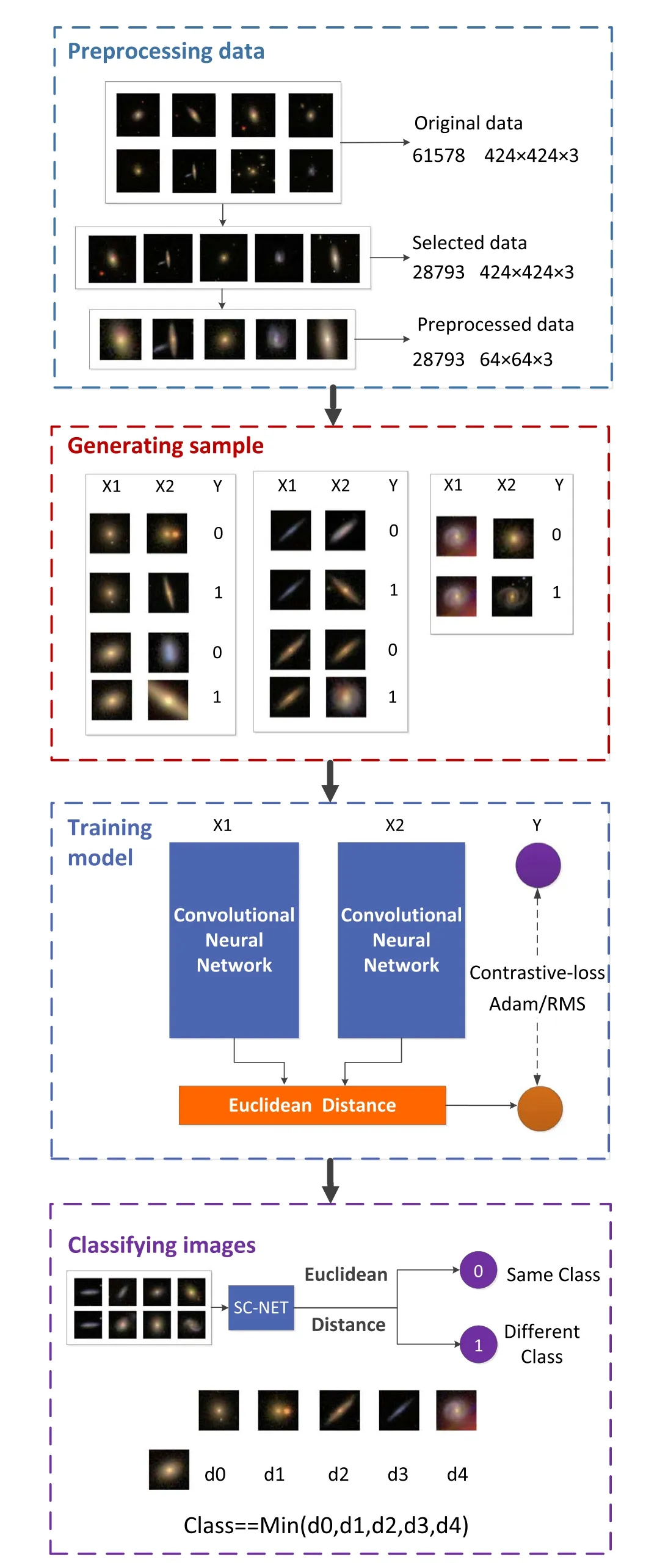
Figure 2.The workflow of the SC-Net model,including data preprocessing,sample generating,model training,and image classifying.

Figure 3.Data processing for the image (ID 11,244) from 424×424 to 64×64.

Figure 4.Images sample from five categories.

The feature extraction module consists of six convolutional layers and two fully connected layers,details are shown in Table 3.The convolutional layers all use 3×3 convolutional kernels.To avoid overfitting,we inserted BatchNormalization layers following each convolution layer,which shrinks the neuron inputs to a normal distribution with a mean of 0 and a variance of 1,rather than a wider random distribution.After every two convolution layers,maximum pooling and dropout layers are added to reduce input data size for the next block.Details of the maximum pooling layers are given in Section 3.1,and the essence of dropout layers is to randomly discard a certain number of neurons to improve the generalization ability of the model.The output of the fully connected layer is a feature vector in the form of 128×1,which will be passed to the second part for the distance calculation.

The Euclidean distance of two feature vectors is given by

where xiis the ith element of the first feature vector x,and yiis the ith element of the second feature vector y.When Dvis less than 0.5,the two images are identified to be sufficiently similar,then classified to be “from the same category.” Otherwise,the images are classified to be“from different categories.”Overall,one needs to train about 9 million parameters in the entire SC-Net model,including the modules of feature extraction and classification.

4.3.Implementation Details

The hardware system utilized in this study contains:Intel(R)Core(TM) i5-9300H CPU @2.40 GHz 2.40 GHz;NVIDIA GeForce RTX 2060 6 GB.Software environment comprises python 3.7.3,Keras 2.3.1,NumPy 1.16.2,Matplotlib 3.0.3,OpenCV 3.4.2.16.The total runtime is about 128 h for ten replicates of 30 experiments.

In each epoch,the batch-size is set to 32;the loss function is contrastive-loss introduced in Section 3.2;the optimizers adopted in the methods based on CNNs are Adam,while we use both Adam and rms for the SC-Net;the initial learning rate is 0.01,which decreases by ten every ten iterations.Each group experiment was iterated 100 times,and the chosen model was selected according to the ACC and Loss curve.Figure 6 shows ACC and Loss curves of the SC-Net model under the Adam optimizer and 20,000 samples in the data sets,we choose a model between 40 and 50 epochs because,at that time,the distance between the validation-loss and training-loss begins to grow,and validation-loss becomes stable,as descried in Figure 6(a).Likewise,the chosen models based on deep CNNs are selected between 30 and 40 epochs,and the chosen model based on the SC-Net with rms optimizer is selected between 50 and 60 epochs.

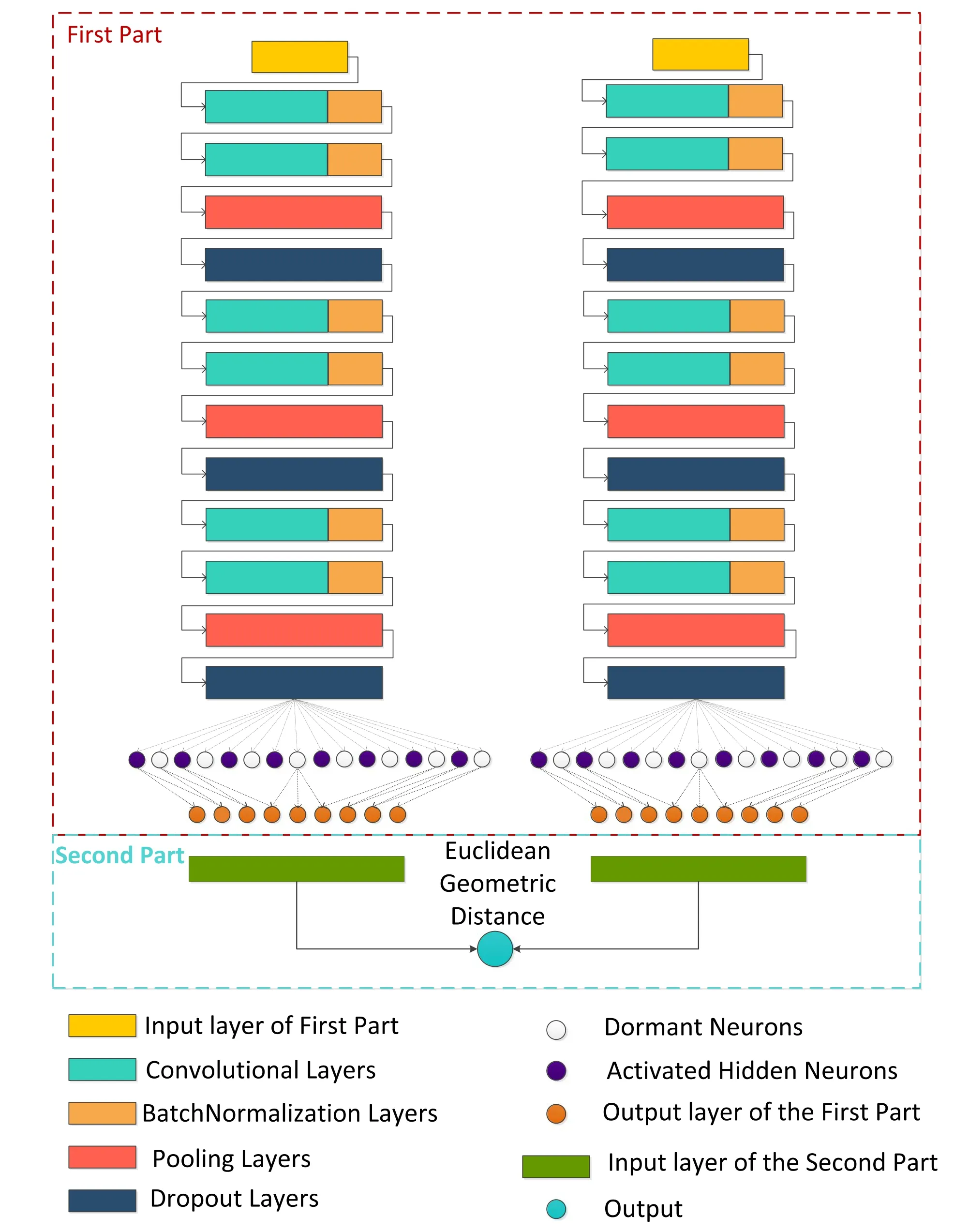
Figure 5.Architecture of the SC-Net model.The meaning of each icon is explained at the bottom of the figure.

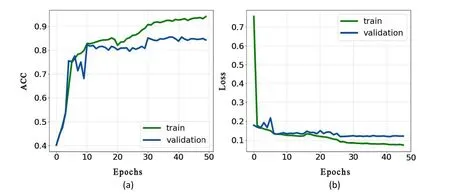
Figure 6.The ACC (a) and Loss (b) curves of the SC-Net model under the Adam optimizer with 20,000 samples in the data set.In 30 groups of experiments,the iteration times of each experiment was determined according to this figure.We chose the position between 40 and 50 where val-loss gradually flattened with iteration time increasing.

5.Results

The experiment is performed under six data sets and five models,including three traditional CNNs (AlexNet,VGG_16,ResNet_50) and two SC-Net models,i.e.,30 experiments in total.Specifically,the sizes of training sets are 1000,5000,10,000,15,000,20,000 and 28,793,respectively.The details of organizing the data sets with different sizes are introduced in Section 2.The five methods are AlexNet,VGG_16,ResNet_50,SC-Net rms,and SC-Net Adam.We adopt accuracy(ACC)as the metric for quantifying the classification performance,which is defined as

where NTPstands for the number of true-positives,NTNstands for the number of true-negatives,NFPdenotes the number of false-positives,and NFNdenotes the number of false-negatives.

As is shown in Table 4 and Figure 7,the SC-Net model achieves the highest accuracy results with all experimental data sets.The most significant gap is 21% compared to AlexNet when the training set contains 1000 images.Considering the results displayed in Figure 8,when the training set size is 28,793,the ACC of SC-Net is 6%higher than that of AlexNet,one can conclude that less training data lead to more significant excellence of the SC-Net model.This reveals the superiority of the SC-Net model compared to traditional CNNs because the SC-Net model takes paired images and labels (Krizhevsky et al.2012;Simonyan &Zisserman 2014;He et al.2015),but the CNNs take images and labels directly.Taking paired images and labels enlarges the size of data sets and magnifies the difference between the images from different morphological categories.In addition,the ACC given by the SC-Net rms method trained by 10,000 images is as high as that given by ResNet_50 trained by 28,793 images.If one plans to acquire a classification ACC of no less than 90%,the SC-Net model needs～6300 images for training,while ResNet_50 requires～13,000 images.The reduction of the requirements of training sets enables the usability of the SC-Net model to detect rare objects (such as strong lenses) potentially.

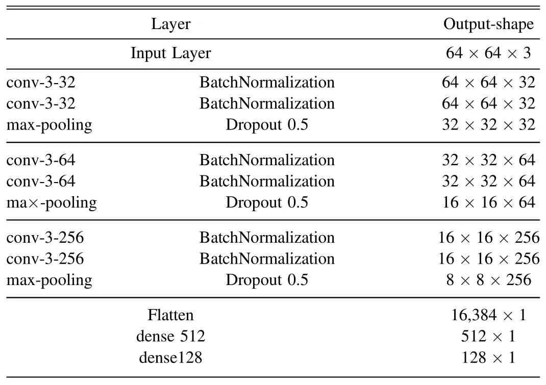
Table 3 SC-Net Structure in Feature Extraction Process

Table 4 30 Groups of Experiments,Each Group of Experiments was Carried out 10 Times,and the Median and Standard Deviation were Taken as the Final Results

We additionally explore the dependence of the classification performance of the SC-Net model on the characteristics of the data.Figure 8 presents the confusion matrix of the SC-Net model,which shows that the SC-Net model can achieve 97.85%,97.34%,and 98.50% ACC in the three categories of completely round smooth,in-between smooth,and spiral,because these galaxies have well-identified features.However,the ACC decreases to 78.33%and 82.59%for cigar-shaped and edge-on galaxies because of their similarity in the case of the Point Spread Functions (PSFs) of SDSS.As is mentioned above,the SC-Net model takes paired images and labels to measure their similarity.Thus,its performance may be suppressed when the features of categories are alike.Expectedly,this issue will be less noteworthy when the image qualityis improved.For instance,with the data from space-born telescopes,smeared substructures in galaxies will be well resolved,such as bugles,disks,and clumps.Then,the SC-Net model can still separate the cigar-shaped and edge-on galaxies.

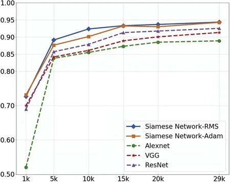
Figure 7.Comparison of experimental results of five methods of ACC.The vertical axis represents the classification performance,the horizontal axis represents the size of the data set,and the broken lines with different colors represent different methods.

Moreover,we draw Figure 9 to analyze the correlation between the classification predictions and the distance between testing images and those in different categories in the training sets in feature space.Five panels,(a),(b),(c),(d),and(e),stand for that:the images listed along the column are completely round smooth,in-between smooth,cigar-shaped,edge-on,and spiral,respectively.The values describe the similarity between the images in the columns and rows.The smaller the value is,the more similar the two images are.In each panel,the first row shows an example of correct classification;the second row shows an example of incorrect classification.Blue boxes denote the ground truth,and fonts in red represent the predicted labels.When the classification is correct in the three categories with apparent features,the similarity between the testing and training images in the corresponding category is quite different from that between the testing images and training images in other categories.For instance,the similarity score in Figure 9(a) is 0.06 in the case of correct classification,while the other distance of feature space scores are above 0.80.However,for the types of cigar-shaped and edge-on galaxies,the differences are only 0.005 and 0.036,which can be calculated by 0.116–0.111 and 0.465–0.429,see panel (c).These outcomes further prove that similarity between the data points in different categories in the training set considerably influences the accuracy of galaxy morphology classification.Hence,it is critical to organize training sets sensibly to avoid such similarities as much as possible when one plans to adopt the SC-Net to solve their problems.

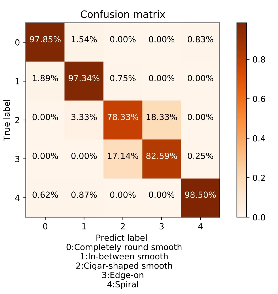
Figure 8.Confusion matrix for classifciation results.The ordinate is the real category of the data,and the ordinate is the category predicted by the model.The diagonal lines represent the percentage of correctly predicted data in each category.The remaining values represent the percentage of predictions that were wrong.

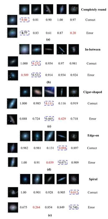
Figure 9.The illustration of the distance of feature space between images measured by the SC-Net.Here(a)–(e)stand for that,the images listed along the column are completely round smooth,in-between smooth,cigar-shaped,edgeon,and spiral,respectively.The values describe the similarity between the images in the columns and rows.The smaller the value is,the more similar the two images are.In each image matrix,the first row shows an example of correct classification;the second row shows an example of incorrect classification.Blue boxes denote the category of the data itself,and the fonts in red represent the category predicted by the SC-Net model.

6.Discussion and Conclusions

Traditional supervised deep learning methods are currently the mainstream for the morphological classifciation of galaxies,which request a considerable volume of training sets.Suppose it demands simulations to create suffciient training sets,which potentially brings model-dependence problems.Thus,we introduce few-shot learning based on the SC-Net model to avoid these drawbacks.Our results present that few-shot learning reduces the requirement of the size of training sets and provides an effciient way to extend the coverage of the training sets in latent space,which can be used to avoid the model-dependence problem.

To illustrate the improvements of our method,we conduct comparative experiments between few-shot learning and approaches based on traditional CNNs,such as AlexNet,VGG_16,and ResNet_50.The results show that few-shot learning achieves the highest accuracy in most cases,and the most significant improvement is 21% compared to AlexNet when the training sets contain 1000 images.In addition,to guarantee the accuracy is no less than 90%,few-shot learning needs～6300 images for training,while ResNet_50 requires～13,000 images.The request for fewer training data can avoid simulation as much as possible when constructing training sets,which bypasses the model dependence problem.Further,suppose we design a recursive strategy to enlarge the training set for galaxy morphology classification by starting with a small training set.Then,few-shot learning can start with extensively fewer data points with known labels than those based on traditional CNNs,which remarkably decreases the workload on creating the primary training set,especially for the case of labeling images by human inspection.

Notably,the performance of few-shots learning is sensitive to the similarity between the images with different labels,though it is still better than that of the methods based on CNNs.For instance,the classification accuracy of completely round smooth,in-between smooth,and spiral are higher than that of cigar-shaped and edge-on.Specifically,the classification accuracy reaches 97.85%,97.34%,and 98.50% in completely round smooth,in-between smooth,and spiral.However,in the two categories of cigar-shaped and edge-on,the accuracy is 78.33% and 82.59%,respectively.It is reasonable because the SC-Net adopts the Euclian distances between images in latent space as the classification metric,while higher similarity leads to shorter distances,which causes mis-classification.This issue is primarily due to the limitation of Galaxy Zoo images observed by ground-based telescopes,presenting few smallscale structures because of large PSFs.After all,the difference between cigar-shaped and edge-on is also hard to identify by human inspection.Expectedly,future high-quality images with detailed structures captured by space-born telescopes can improve the classification performance significantly.

In summary,this study presents the feasibility of few-shot learning on galaxy morphology classification,and it has certain advantages compared to traditional CNNs.Next,we plan to apply the method to observations such as DESI Legacy Imaging Surveys,15https://www.legacysurvey.org/the Dark Energy Survey,and the Kilo-Degree Survey.16https://kids.strw.leidenuniv.nl/Also,to further improve the performance of this approach,we will optimize its architecture and hyperparameters while implementing the above applications.Besides,considering the characteristic of the SC-Net,few-shot learning can also be utilized to identify rare objects,e.g.,merging galaxies,ring galaxies,and strong lensing systems,which draws our interests intensively as well.

Acknowledgments

The data set used in this work is collected from the Galaxy-Zoo-Challenge-Project posted on the Kaggle platform.We acknowledge the science research grants from the China Manned Space Project with No.CMS-CSST-2021-A01.Z.R.Z.,Z.Q.Z.,and Y.L.C.are thankful for the funding and technical support from the Jiangsu Key Laboratory of Big Data Security and Intelligent Processing.The authors are also highly grateful for the constructive suggestions given by Han Yang and Yang Wenyu for improving the manuscript.