Gauss quadrature based finite temperature Lanczos method

Jian Li(李健) and Hai-Qing Lin(林海青)

Beijing Computational Science Research Center,Beijing 100193,China

Keywords: exact diagonalization,Lanczos method,orthogonal polynomials

1. Introduction

In the study of quantum many-body systems, the exact diagonalization (ED) method is intensively used to calculate static and dynamic quantities.[1–4]Since the dimension of many-body Hilbert space increases exponentially with system size, ED is only appliable on systems of relatively small size.But ED is still an effective method since it can always get unbiased result compared with other variational methods like density matrix renormalization group,[5–7]and does not suffer from sign problem in quantum Monte Carlo simulations.[8–10]To solve the problem of large matrix dimension, ED is often based on algorithms from sparse matrix calculation,especially Lanczos method[11–14]and kernel polynomial method(KPM).[15–18]

The Lanczos method is originally used in the calculation of ground state properties, since only extreme eigenvalues and eigenvectors converge well. With the introduction of finite temperature Lanczos method (FTLM) by Jakliˇc and Prelovˇsek,[19,20]finite temperature static and dynamic quantities can be calculated accurately. In FTLM, the true HamiltonianHis represented by an effective Hamiltonian ˆHin the Krylov subspace generated by Lanczos iteration. Then by expanding exp(-βH) into Taylor series, the calculation is reduced to evaluating quadratic forms of the type〈n|HkBHlA|n〉,which can be achieved using effective Hamiltonian ˆH.

KPM is another method used in the calculation of finite temperature properties. The main idea behind KPM is using Chebyshev polynomials to expand quantities like density of states, static and dynamic correlation functions. KPM converges very well at high temperature. But when temperature comes to zero,the low lying states,which KPM does not calculate very accurately,contribute an important part in thermodynamic quantities. To overcome this, the KPM should run several Lanczos iterations to get accurate low lying states,and projects these states out in later calculations. Despite the inaccuracy at low lying states, KPM is believed to be simpler and faster than Lanczos method,and does not suffer from the problem of losing orthogonality occurred in high order Lanczos iteration.[15]

Recently there have been numerical experiments benchmarking the accuracy of FTLM and KPM,[21,22]but the relationship between these two classes of ED methods has not been well explored yet. In this paper, we develop and formulate FTLM in the framework of Gauss quadrature and orthogonal polynomials. In this framework, the Lanczos iteration in FTLM is regarded as a procedure to generate a series of orthogonal polynomials by which different functions of Hamiltonian is expanded. These orthogonal polynomials play the same role as that of Chebyshev polynomials in KPM.The combination of Gauss quadrature and Lanczos iteration has been used in the matrix computation community,[23,24]for example,to give error estimate of solution of linear equations,which is related to the quadratic formsu†A-iufori= 1,2.Here we generalized this method to the calculation of more general formu†f(H)Ag(H)v,which needs the notion of twodimensional Gauss quadrature and can be applied in the calculation of finite temperature dynamic correlation functions.This Gauss quadrature based framework fills the conceptual gap between FTLM and KPM, which makes it easy to apply orthogonal polynomial techniques commonly used by KPM in the FTLM calculation. The implementation of FTLM is reduced to one-or two-dimensional Gauss quadratures,which is similar to that of KPM, and is simpler than the procedure of Taylor series expansion.

2. Fundamental theory

In large scale exact diagonalization of quantum manybody systems, the HamiltonianHis given as a sparse Hermitian matrix of dimensionN. Usually the study of static and dynamic quantities involves calculating trace off(H), wherefis a smooth function. For example,f(H)=exp(-βH)for the calculation of partition function, andf(H)=exp(-iHt)for the calculation of real time evolution. As we will see in Section 3, we can get many static and dynamic quantities by a suitable choice off(H), and an effective way to calculate following quantities:

1.u†f(H)u,

2.u†f(H)vwhereu/=v,

3.u†f(H)Ag(H)v.

HereuandvareN-dimensional vectors representing quantum many-body states. As developed in following sections,the first quantity is related to one-dimensional Gauss quadrature,and the second and third quantities can be calculated by two-dimensional Gauss quadrature.

2.1. Weighted summation and Gauss quadrature

LetHbe a Hermitian matrix of dimensionNwith following eigenvalue decomposition:

We can see thatu†f(H)ucan be seen as a weighted summation with weightswi=|(X†u)i|2and evaluation pointsλibeing the eigenvalue ofH. This form is exactly the same as that of Gauss quadrature,[25]which is extensively used in numerical calculation of integrals.

To be more specific, Gauss quadrature is an approximation method to calculate integrals numerically. It transforms the integral into a weighted summation

To validate the algorithm of FTLM above, we need to dig into the mathematical principles behind Gauss quadrature,which leads us to the theory of orthogonal polynomials. Furthermore,theory of orthogonal polynomials can give error estimates of FTLM,which is essential in numerical simulation.

2.2. Theory of orthogonal polynomials

The theory of orthogonal polynomials[27]is fundamental in the implementation and analysis of Gauss quadrature.Given interval(a,b),define inner product of any two functionsfandgin(a,b)as

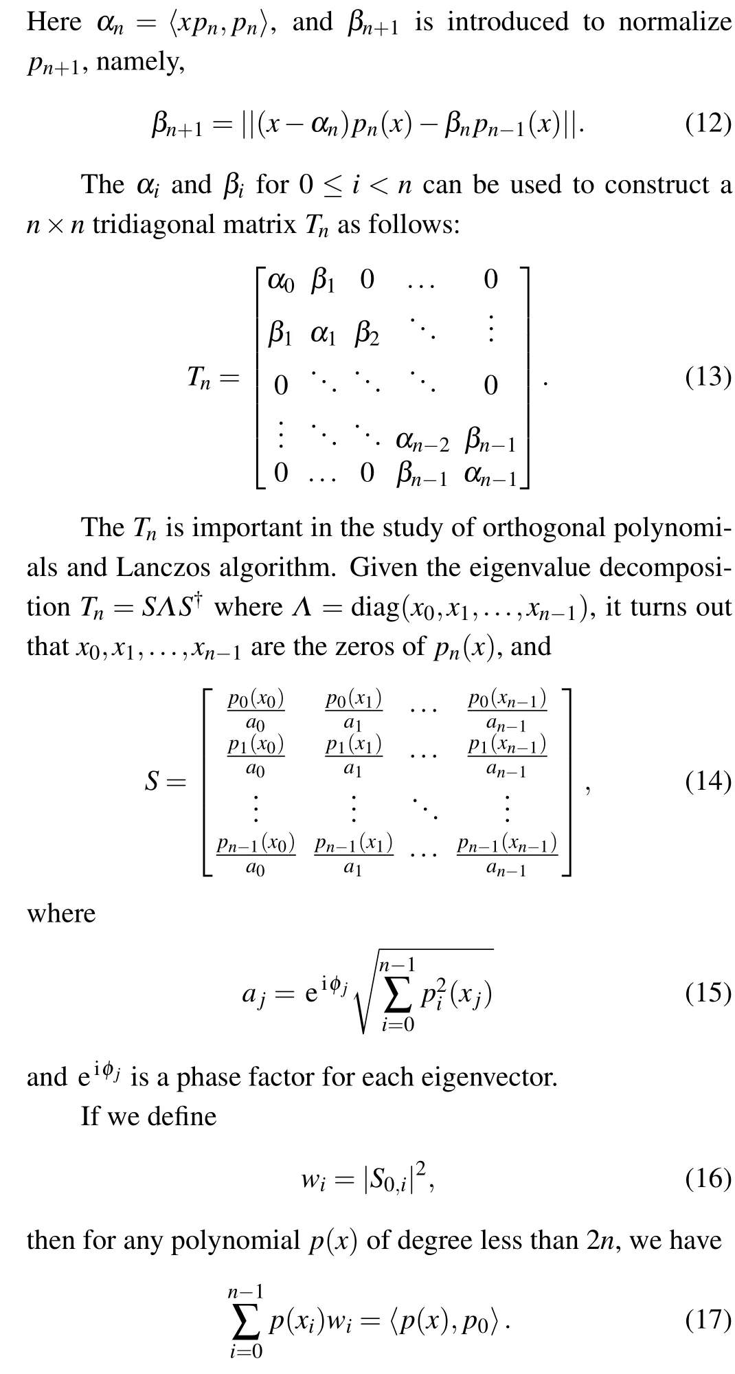
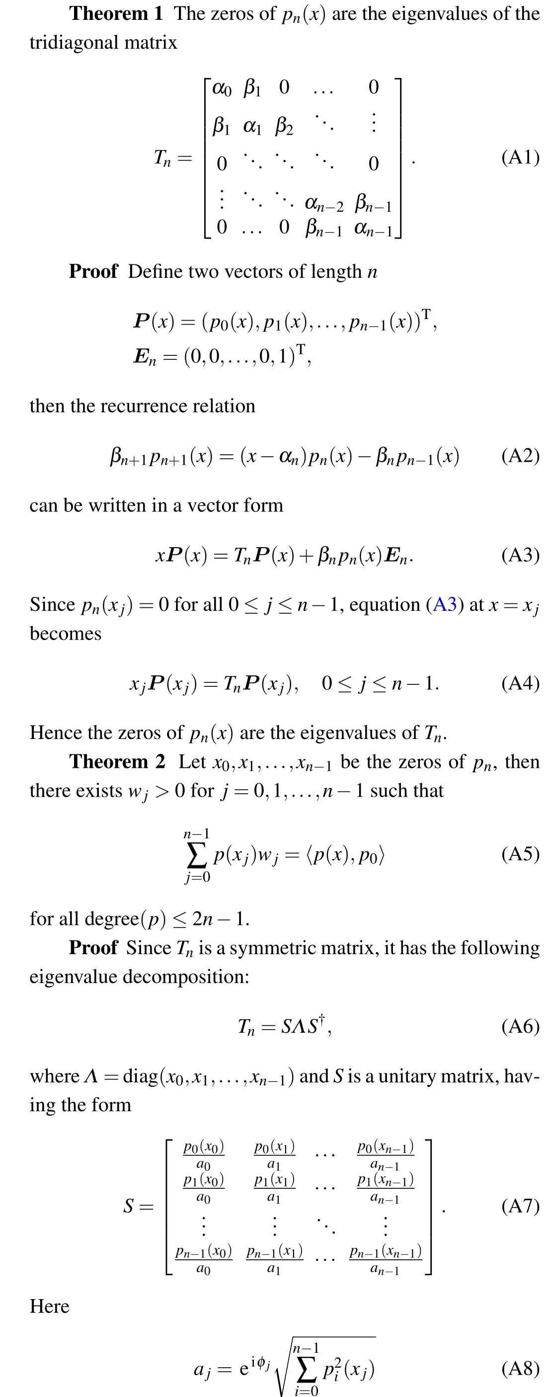
Equation(17)is the fundamental result of Gauss quadrature, which states that we can choose a set ofnnodes and weights to construct a quadrature rule of order 2n-1. One can find detailed proof of Eqs.(14)and(17)in Appendix A.

We can restate Gauss quadrature in the language of discrete inner product. Given the nodesxiand weightswidefined above, we can define a discrete inner product in [a,b] and its associated norm by

2.3. Relationship with Lanczos iteration

Lanczos iteration is a standard method to transform a Hermitian matrix into tridiagonal form by an unitary transformation. For a given matrixHand a starting normalized vectoru,the Lanczos iteration is given by

The transformed tridiagonal matrix is exactly the same asTndefined in Eq.(13).

We can see many similarities between Eqs.(11)and(21).Actually Lanczos iteration does its transformation according to a sequence of orthogonal polynomials.[24]To see this, let us defineqi=pi(H)q0,wherepiis a polynomial of degreei.According to Eq.(21),we have

which is the same recurrence relation ofpnin Eq.(11).

Here for simplicity we assume that for the Hermitian matrixHof dimensionN, we can transform it into a tridiagonal matrixTNof the same dimension by Lanczos iteration with a suitable normalized starting vectoru. Note that Lanczos tridiagonalization procedure is generally an unitary transformation,namely,

which is the same weight as that of Gauss quadrature in Eq.(16).

Now we can explain more explicitly the algorithm of FTLM in Subsection 2.1 using the language of discrete inner product. Supposefis a smooth function anduis a normalized vector,by definition,we have

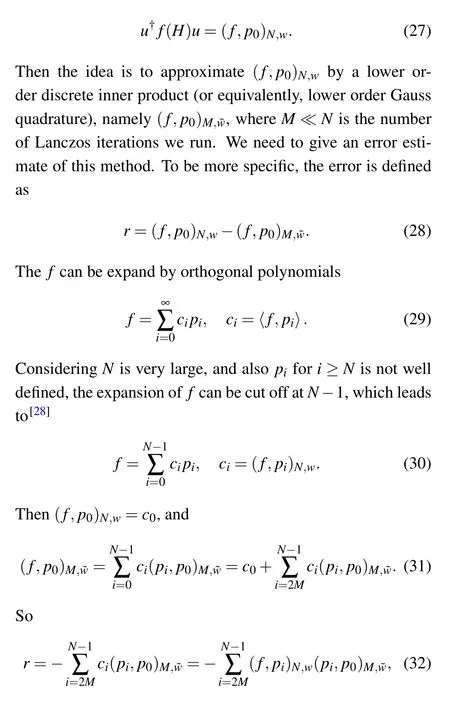
which means thatMLanczos iterations will give approximation up to order of 2M.

2.4. Two-dimensional Gauss quadrature

Here comes to the question of how to calculate the following quantities:

1.u†f(H)vwhereu/=v,

2.u†f(H)Ag(H)v.

We can see that the second quantity is a general form of the first one givenA=g(H)=1. As for the first case, ifu,vare real vectors andHis a real symmetric matrix,we can use the following identity[23]to calculateuT f(H)v:

Then we can use the method talked before to calculateuT f(H)v, the only difference is that we need to run Lanczos iteration twice.

But for the general case, namely,u†f(H)Ag(H)v, we need a different method, which needs the notion of twodimensional Gauss quadrature,as will be discussed below.

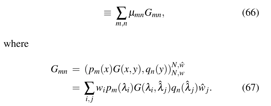
Two-dimensional Gauss quadrature, and also twodimensional orthogonal polynomials, can be easily constructed from a tensor product of two one-dimensional Gauss quadratures and orthogonal polynomials respectively. Formally,given two weighted Hilbert spaceL2w(a,b)andL2ˆw(a,b),we can construct a Hilbert space on(a,b)×(a,b)by defining the following inner product:

in which we have introduced an auxiliary functionC(x,y). It is only defined at some discrete points as follows:which means that we only need to run one Lanczos iteration forM1steps. In general case,the numerical effort for the calculation ofμmnranges betweenN(M1+M2)andNM1M2operations,depending on whether memory is available for savingM1(orM2)vectors of dimensionN.

3. Formulas for static and dynamic quantities

Until now we have not discussed how to calculate static and dynamic quantities for a real quantum system. Actually the routines in FTLM share many similarities as in KPM,[15,17]thus can be expressed in a unified form.

In this section and later Dirac bra–ket notations will be used to denote matrix vector multiplication, this notation is inconvenient in previous sections but more suitable when it comes to physical applications.

3.1. Stochastic evaluation of traces

Although we have the method to calculate〈u|f(H)|u〉,in many cases we need to evaluate the trace of a given operator.For example,the partition function is given by a trace

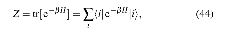
where{|i〉}is a complete set of basis.

At first glance it seems impossible to evaluate since the Lanczos iteration needs to be repeated for allNstates of a given basis, which makes the total computational effort proportional toN2. It turns out that extremely good approximation of the trace can be obtained with a much simpler approach: stochastic evaluation of trace, in which estimate of trace is based on the average over a small numberR ≪Nof randomly chosen vectors[15,30]

Typical chosen ofξrican be Gaussian distribution with average 0 and standard deviation 1.

3.2. Thermal average and density of states

Given partition functionZ=tr[e-βH], the thermal average of operatorAis

We can use stochastic evaluation of traces to calculate these quantities. From Eq. (43) we can see that only one Gauss quadrature rule is need to calculate both〈r|e-βH|r〉and〈r|e-βHA|r〉for each given random vector|r〉, so only one Lanczos iteration is need for the given random vector. This can be generalized to many operators if we want to calculate thermal average of these operators at the same time.

Here we consider two limiting cases to illustrate the accuracy of FTLM.

1.β →0. This is the high temperature limit,where

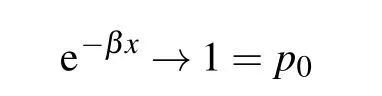
and according to Eq.(32),few Lanczos iteration will give accurate result.

2.β →∞. This is the low temperature limit, e-βxwill be sharply dominated atx=Emin. From the theory of orthogonal polynomial expansion, many high order expansion will contribute to this nearly discontinuous function. Furthermore,Gibbs oscillation[17,31]will creep into the expanded function,which introduces numerical instability. In this case,low temperature Lanczos method[32]have been proposed to address this problem. One can also use ground state Lanczos method in this super low temperature regime,which is generally more accurate.

As for density of states,it is defined as

3.3. Real time evolution

As a studying case,here we consider real time evolution.Specifically,we are interested in the quantity

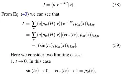
equation(59)is accurate for very few Lanczos iteration.

2.t →∞. In this case both sin(tx) and cos(tx) will oscillate badly in the integration interval[Emin,Emax],and Gauss quadrature based integration rule will fail to converge.

So the real time evaluation is different from imaginary time evaluation in the sense that real time evaluation will fail to converge in thet →∞limit, while imaginary time evaluation will admit accurate results in bothβ →0 andβ →∞limits.

3.4. Dynamic correlation function

Before we dig into the calculation of finite temperature correlation function, we may first give a glance for the zero temperature case. For zero temperature,the dynamic correlation function for two operatorAandBis

in which the term〈r|e(-β+it)HAe-iHtA|r〉follows the general form〈u|f(H)Ag(H)|v〉withf(x;t)= e(-β+it)xandg(x;t)=e-itx, and needs a two-dimensional Gauss quadrature to calculate.

As mentioned in real time evolution, Gauss quadrature based FTLM is not accurate for evolution timetbeing large,this is also true in Eq.(61). In this case it is better to calculate the Fourier transform ofC(t)

4. Numerical results of 1D XY model

In this section we give numerical results to illustrate the idea of Gauss quadrature based finite temperature Lanczos method. The numerical calculation is carried out on the onedimensionalXYmodel.

TheXYmodel is introduced by Lieb,Schultz and Mattis in 1961,[33]they considered a chain ofN1/2-spins,governed by the Hamiltonian

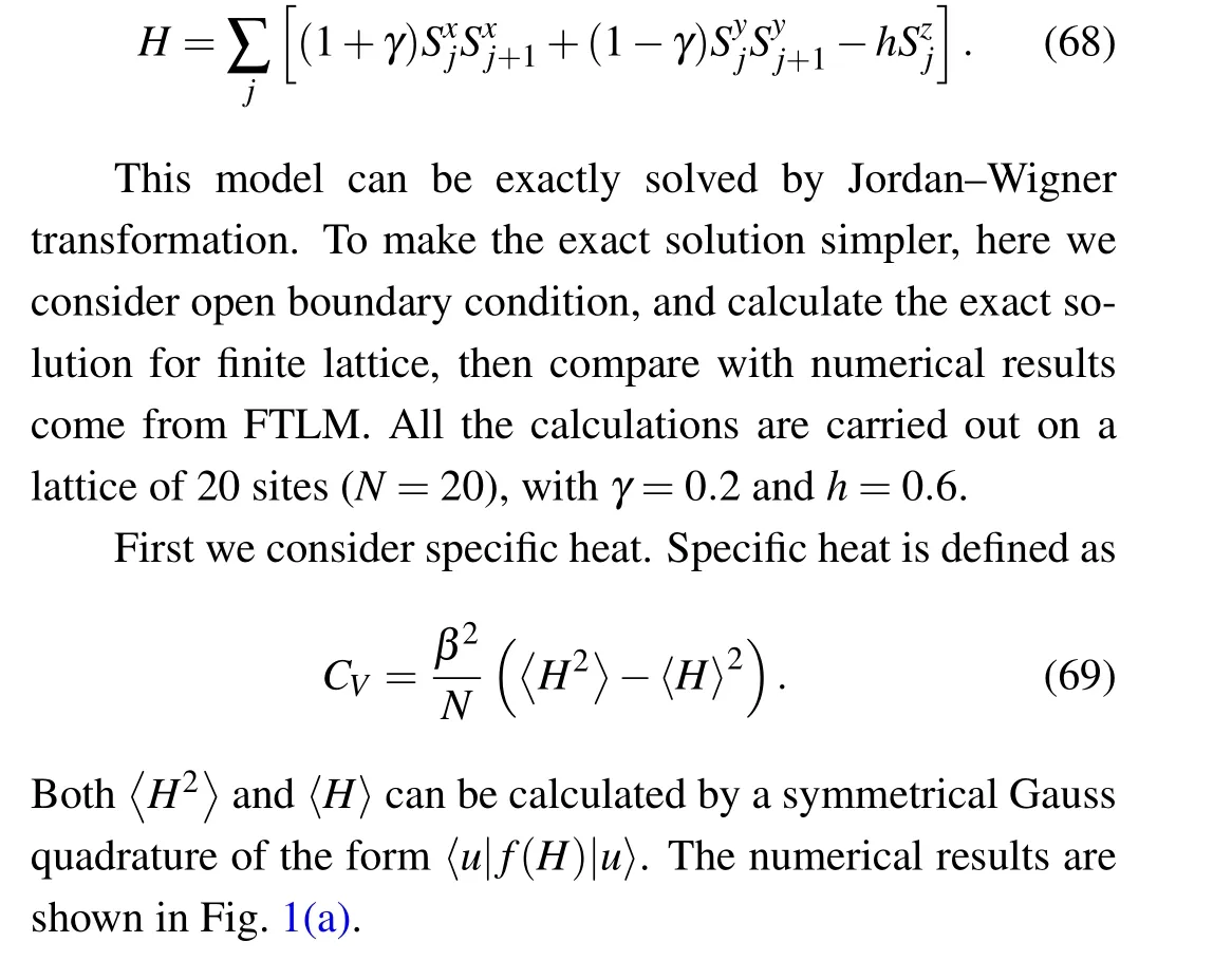
Fig.1.(a)specific heat and(b)magnetic susceptibility of 1D XY model.In both figures the Lanczos iteration steps is set to 100,and the number of random vectors(denoted by R)is set to 20 and 100 respectively.

The second quantity we consider is magnetic susceptibility,which is defined as Both〈m2z〉and〈mz〉can be calculated by an unsymmetrical Gauss quadrature of the form〈u|f(H)|v〉. The numerical results are shown in Fig.1(b).

The computational effort to calculateCVandχare approximately same,since only one Lanczos iteration is needed to calculate the symmetric Gauss quadrature〈u|f(H)|u〉and the unsymmetrical Gauss quadrature〈u|f(H)|v〉. In both case the Lanczos iteration steps is set to 100,and the number of random vectors(denoted byR)is set to 20 and 100 respectively.From Fig.1 we can see that FTLM is accurate at high temperature, while the accuracy at low temperature is influenced by statistical fluctuations from random vectors.

The third quantity we calculate is the dynamic correlation function of the average magnetization inzdirection,[34]which is defined as

This quantity can be calculated by a two-dimensional Gauss quadrature of the form〈u|f(H)Ag(H)|v〉. The numerical results are shown in Fig.2(a).

We can see that numerical result agrees well with exact result whent ＜10. But for lagert, the numerical result is very inaccurate. As discussed in real time evolution(see Subsection 3.3), Gauss quadrature based integration will fail to converge for highly oscillate functions such as eitHfor larget.

It is usually more convenient to study the Fourier transform ofχ(t)defined as follows:

The numerical results are shown in Fig.2(b).

The calculation ofχ(ω) also involves two-dimensional Gauss quadrature in which the Diracδfunctions are replaced by Lorentz functions(see Eq.(65)). Since the time scale that FTLM can accurately calculate can not be large, the resolution inωspace, which is represented by the parameterεin Lorentz function,is also limited due to the time-energy uncertainty principle. As shown in Fig.2(b),the parameterεis set to 0.01. Smallerεwill lead to negativeχ(ω) values, which indicates the failure of convergence.

5. Conclusion

This paper has shown the tight relationship between Lanczos algorithm and orthogonal polynomials, and developed finite temperature Lanczos method in the framework of Gauss quadrature. The Lanczos algorithm can be regarded as a procedure to generate a series of orthogonal polynomials by which different functions of HamiltonianHare expanded.These orthogonal polynomials also define Gauss quadrature rules.The nodes and weights of Gauss quadrature are given by the eigenvalues and eigenvectors of tridiagonal matrix which is generated by the Lanczos iteration.Given the Gauss quadrature rule,the calculation of quadratic formu†f(H)u,which is the main part of finite temperature Lanczos method, can be reduced to a one-dimensional Gauss quadrature. The calculation of more general formu†f(H)Ag(H)vcan be reduced to a two-dimensional Gauss quadrature. Then we showed that many finite temperature static and dynamic quantities can be calculated by one-or two-dimensional Gauss quadratures.

Our development of FTLM is not to improve numerically the original FTLM introduced by Jakliˇc and Prelovˇsek, since both methods admit same numerical results. The advantage of this Gauss quadrature based framework is that it fills the conceptual gap between FTLM and KPM, and makes it easy to apply orthogonal polynomial techniques commonly used by KPM in the FTLM calculation. One unexplored extension of this framework is applying different kernels in FTLM to reduce Gibbs oscillation in the expansion of incontinuous functions. We believe that after this development,FTLM will find more applications in the calculations of quantum many-body systems.

Appendix A: Two theorems on orthogonal polynomials

Acknowledgements

This work is supported by the National Natural Science Foundation of China (Grant Nos. 11734002 and U1930402).All numerical computations were carried out on the Tianhe-2JK at the Beijing Computational Science Research Center(CSRC).