Inferring interactions of time-delayed dynamic networks by random state variable resetting

Changbao Deng(邓长宝), Weinuo Jiang(蒋未诺), and Shihong Wang(王世红)

School of Sciences,Beijing University of Posts and Telecommunications,Beijing 100876,China

Keywords: time delays,network reconstruction,random state variable resetting

1. Introduction

Complex dynamic networks are used to model interacting individuals in interdisciplinary research.[1-6]Due to the limited propagation speed of signals, time delays play a significant role and exist extensively in real systems.[7-11]Detecting the interactions in networks is helpful for understanding the collective behaviors of complex systems. However,due to systematic nonlinearity,noises,a lack of information,time delays,and so on,inferring the interactions in dynamic networks is complicated and challenging.Some methods have been proposed for inferring the interactions without time delays. Typical statistical methods,such as cross correlation,[12]Granger causality,[13]mutual information,[14]and transfer entropy,[15]are usually used to define functional connections, which provide limited information for interacting nodes.In recent years,researchers have explored approaches to inferring the interactions by solving ordinary differential equations (ODEs).Some detection methods can be used to reconstruct a linear dynamic network,[16-19]while expanding basis[20-24]and expanding variable[25,26]methods are proposed to detect a general nonlinear dynamic network. These methods not only reveal connections, but also provide information on local dynamics and coupling functions.For these methods,[20-26]solving ODEs requires the output data of the whole network. The existence of noises increases the difficulty of network reconstruction, sometimes, also leading to new approaches.[27,28]In Refs. [27,28], the injection of noise into the nodes enhances the target interaction and weakens the effect of hidden nodes and variables. In addition, there are some proactive methods, such as driving-response controlling,[3]copysynchronization,[3]and random phase resetting.[29]

For time-delayed dynamic networks, accurately identifying delays is the prerequisite for network reconstruction. There are several existing methods for identification of time delays, such as parameter estimation,[30]adaptive synchronization,[31,32]model-fitting approaches,[30,31]perturbation methods,[32,33]the permutation-information-theory approach,[34]and cross map evaluation.[35]However,most of these methods are appropriate in a single dynamic system. In a dynamic network, a large number of time-delayed interactions make network reconstruction extremely difficult. Recently, Zhanget al.proposed a new method to detect time delays and the average coupling strengths through the correlations induced by fast-varying noises(here called FVN).[36]

The random state variable resetting(RSVR)[37,38]method proposed by Shiet al.,as an active control method,can be used to detect the interactions in dynamical networks. By randomly resetting the state variable of a driving node, the influence of other nodes and variables on a response node can be simplified as background average and fluctuations, and then the equivalent coupling function of a driving node to a response node can be reconstructed using only the data of two related nodes.In this paper, we introduce the RSVR method to reconstruct time-delayed dynamic networks. Based on the output data after randomly resetting, we define the nearest neighbor correlation (NNC) function for a given time delay. According to the increment of the defined NNC at the actual time delay,we can identify the time delay accurately.The error of determined time delays only depends on the sampling time interval. Compared with the FVN method,[36]the NNC function defined through RSVR is effective even for a relatively low sampling frequency. After the time delay is determined, the equivalent directed time-delayed coupling function can be reconstructed from measurable data. By arbitrarily resetting the variable of a driving node, the RSVR method can infer the time delays and equivalent directed time-delayed coupling functions of the driving node to the other response nodes. In actual networks,some nodes and variables are not measurable.This reconstruction method is applicable to networks with hidden nodes and variables.

2. Method

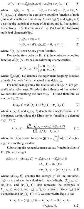
To determine the time delay of nodejto nodeiin Eq.(1),we first define the nearest neighbor correlation (NNC) function with the time delayτas

3. Simulation results

3.1. Time-delayed coupled Lorenz networks

First, consider a time-delayed coupled Lorenz network[39]

We assume that variablexiis measurable and variablesyiandziare unmeasurable. We randomly reset variablex1distributed uniformly within [-20,20] and acquire the data Eq.(4).Resetting time intervalsτresetare uniformly distributed in[1,2]. Our task is to use these data to infer the time delaysτi1and coupling coefficientsWi1. Selectingi=5,τ51=0.308 is the time delay of node 1 to node 5,andW51=0.944 is the coupling coefficient of node 1 to node 5. Given a sampling interval Δt=0.006,thenτ51=51.33Δt,and thus the discrete delayn51=51. Choosingτ=nΔt, we calculate ˙xi(tm+τ)from measured data by the forward difference ˙xi(tm+τ) =[xi(tm+τ+Δt)-xi(tm+τ)]/Δt. Then we smooth these results via Eq.(9)withM=5×105andd=0.4. The smoothing curves of ˙x5(x1,τ)whenτ=0,0.300(50Δt),0.306(51Δt),0.312(52Δt)are plotted in Figs.1(a)-1(d). In Fig.1(a)(τ=0)and Fig.1(b)(τ=50Δt), the smoothed data display randomness, i.e., no dependence. In fact, whenτranges from 0 to 50Δt,node 5 has not been affected by node 1 due to the time delay; ˙x5(x1,τ)maintains such randomness. Whenτ=51Δt(Fig. 1(c))and 52Δt(Fig.1(d)), the smoothed data display a linear dependence.In Fig.1(c),the graph representsτ=51Δt,you may observe the calculated ˙x5(x1,τ)has already been affected by the reset variablex1. The reason for that is because we are using forward difference. Thus,the affection looks like happen before the real time delayτ51=51.33Δt.

Fig.1. Simulation results of Eq.(22)with linear diffusion coupling functions hij(xi(t),x j(t-τij))=Wij(xj(t-τij)-xi(t)). Data volume M=5×105 and sampling interval Δt =0.006. The actual time delay of node 1 to node 5 τ51=0.308,τ51=51.33Δt,and the discrete time delay n51=51. Left: Smoothing curves ˙x5(x1,τ)for (a) τ =0, (b) τ =0.300 (50Δt), (c) τ =0.306 (51Δt), (d) τ =0.312 (52Δt)vs. the state variable x1. The curves have no dependence on x1 (a), (b) and a linear dependence (c), (d). Right: (e) Dependence of NNC51 on discrete time delay n. The dashed line marks the actual time delay τ51/Δt =51.33. (f) Dependence of NNC41 on n. (g) Reconstructed discrete delays ˆni1 plotted against the actual discrete delays ni1. (h) Reconstructed coupling ˆWi1 plotted against the actual Wi1. (i)Reconstructed ˆnij plotted against the actual nij. (j)Reconstructed ˆWij plotted against the actual Wi j.

We calculate NNC51(n)via Eq.(13),wheren=/Δt」,and the results (circles) are shown in Fig. 1(e). In Fig. 1(e),the dashed line marks the actual time delayτ51/Δt=51.33,which is located between the first non-zero point (n= 51)and the second non-zero point (n= 52). We can observe that NNC51(50)=0, and NNC51(51) and NNC51(52) have a significant increment. The increments originate from the effect of the delay and the forward difference calculation of ˙x5(tm+τ). Here we choose the larger of the two non-zero values,i.e., ˆn51=52 as the reconstructed discrete delay. Ifτij/Δtis not an integer,the maximal error of reconstructed time delay ˆτi j= ˆni jΔtis a sampling interval, where ˆni jis the numerical discrete delay of nodejto nodei. For comparison,we select node 4 and calculate NNC41(n),and the results are presented in Fig. 1(f). Due to no link of node 1 to node 4, the values of NNC41(n)are near to zero and there is no significant increment point. Comparing Fig.1(e)with Fig. 1(f), we conclude that we can determine time delays by random variable resetting via Eq.(13).

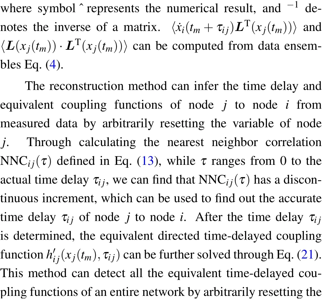
In Fig. 1(g), we plot the curve of numerical ˆni1against the actualni1. The results show that the numerical ˆni1values are consistent with the actual values. After determining the time delays, we can select suitable basesL=[1,x1]Taccording to the linear dependence shown in Fig.1(d),and then coefficientsAi1,1of variablex1are used as estimates of the coupling coefficients ˆWi1, which also show good agreement with the actual coupling coefficientsWi1as in Fig.1(h). Then we randomly selected 20 nodes in the network to reset, and the inferred time delays ˆni jand coupling coefficients ˆWijof these 20 nodes to all nodes are shown against the actual valuesnijandWi jin Figs. 1(i) and 1(j). We can observe that the numerical ˆnijvalues are consistent with the actual valuesni j,but there is some deviation in the numerical coupling coefficients ˆWij. Because of discrete time sampling,the error of detected time delays depends on the sampling interval Δt. The error of detected time delays can cause deviations of interactions and the deviations further make reconstructed coupling coefficients decrease or increase. Therefore,the deviations of determined coupling coefficients depend on specific coupling functions,state variables,and the error of time delays.

We will discuss how the number of resetsMand the sampling interval Δtaffect the reconstruction results. We use the root-mean-square errorsEτandEWto evaluate the reconstruction results ˆτijand ˆWi j,

Figure 2 represents the errors of the calculated time delaysEτ(Fig.2(a))and the calculated coupling coefficientsEW(Fig.2(b)).In Fig.2(a),due to the influence of fluctuationsrij,the errors of time delaysEτare greater for a relatively small number of resetsM. AsMincreases,the reconstruction errorEτreduces until it reaches saturation,which depends on sampling interval Δt. This is because when the amount of data is large enough,the errors of time delays are determined by sampling interval Δtand the maximum deviation of a time delay is less than Δt.In Fig.2(b),we can observe that,as the amount of data increases, the errors of the coupling coefficient decrease until a saturation state is reached. The errors of coupling coefficients mainly originate from sampling interval Δt,thus,to reduce the errors of coupling coefficients,decreasing sampling interval Δtis more effective than increasing the amount of dataM.

In Eq.(22),nonlinear interactions,hi j(xi(t),xj(t-τij))=Wijx2j(t-τij),are considered and the numerical results are represented in Fig. 3. To avoid system divergence, we decrease the coupling coefficientsWi jand they are reduced to one tenth of the original values. We plot the curve of ˙x5(x1,τ) againstx1shown in Fig. 3(a), whileτ=52Δt. NNC51(n) are calculated by using Eq.(13)and the results are shown in Fig.3(b).Figure 3(b)is similar to Fig.1(e),and we can observe that the actual time delayτ51/Δt=51.33 is smaller than the second non-zero point and greater than the first non-zero point. We select the second non-zero point as the numerical discrete delay,i.e., ˆn51=52. Similarly,after determining the time delayτij,we select basisL=[1,x2j]Tand solve the coupling coefficient ˆWij.The curves of Figs.3(c)and 3(d)are similar to those of Figs.1(i)and 1(j).

Fig.2. The root-mean-square error Eτ of reconstruction time delays and the root-mean-square error EW of coupling coefficients are shown in(a)and(b),respectively. (a) Dependence of Eτ on M for Δt =0.002,0.006,0.010, and 0.020. (b)Dependence of EW on M.

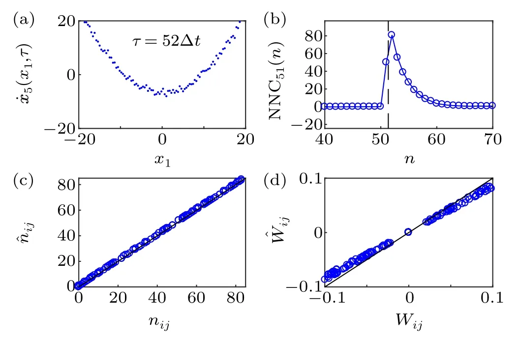
Fig. 3. Simulation results of Eq. (22) with nonlinear coupling functions hij(xj(t-τij),xi(t))=Wijx2j(t-τij). M =5×105 and Δt =0.006,τ51 =0.308. (a) Smoothing curves of ˙x5(x1,τ) plotted against x1 at τ =0.312 (52Δt). (b) Dependence of NNC51 on n. The dashed line marks the actual time delay τ51/Δt=51.33.(c)Numerical ˆni j plotted against the actual nij. (d)Numerical ˆWij plotted against the actual Wij.

3.2. Time-delayed Hodgkin-Huxley neural network

We consider time-delayed Hodgkin-Huxley[40]neural network dynamics,

where the coupling coefficientsWijare uniformly distributed in [0.04,0.2] and [-0.2,-0.04] for excitatory and inhibitory synapses, respectively, andWij=0 for no links. The ratio of excitatory synapses to inhibitory synapses is 4:1. The time delaysτijare uniformly distributed in [0,1.0]. The structure of this network is exactly the same as that of Eq. (22). The parametersVrev=110 mV,Vth=100 mV,andσ=0.01. Gate variablesmi,hi,niare expressed by

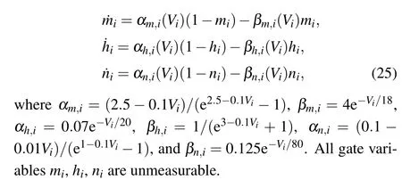
Without loss of generality, we arbitrarily reinitialize the membrane potential of node 1,V1∈[-30,110] withτreset∈[30,40].We set the sampling interval Δt=0.008 and the number of resetsM=105. In Fig.4(a), we plot the curves of the smoothed ˙V5(V1,τ) withτ=0.616 (77Δt). The actual time delay of node 1 to node 5τ51=0.6161 (77.0125Δt). When and only when variableV1exceedsVth=100 mV,neuron 1 has a significant effect on the postsynaptic neuron 5. Similar to as in Fig.3(b),we plot the curves of NNC51(n). The dashed line marks the actual time delayτ51/Δt=77.0125, which is near to the first non-zero point(ˆn51=77). By resetting every node,we infer all discrete delays ˆni jand the results are shown in Fig.4(c).We can see that the reconstructed time delays display satisfactory results. Selecting[1,1/(1+e-(Vj-Vth)/σ)]Tas the basis, estimated coupling coefficients of 1/(1+e-(Vj-Vth)/σ)are ˆW′ij=WijCm,i〈Vrev-Vi〉, with ˆWi j= ˆW′i j/(Cm,i〈Vrev-Vi〉)as the estimates of actualWi j. The results are represented in Fig.4(d). Similar to as in Fig.3(d),the numerical coefficients also have deviation.

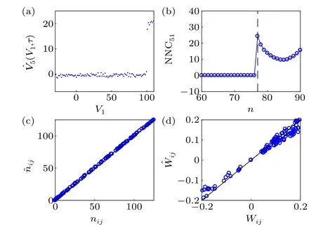
Fig. 4. Simulation results of a time-delayed Hodgkin-Huxley neural network. Set sampling interval Δt =0.008 and the reset number M =105.The actual time delay of node 1 to node 5 τ51 =0.6161 (77.0125Δt). (a)˙V5(V1,τ)plotted against V1 at τ=0.616(77Δt).(b)NNC51 plotted against n. The dashed line marks the actual time delay τ51/Δt =77.0125. (c)Numerical ˆnij plotted against the actual nij. (d)Numerical ˆWij plotted against the actual Wij.

4. Discussion

We can detect the equivalent coupling functions of timedelayed dynamic networks by the random state variable resetting method. To determine the time delayτijof nodejto nodei, we define the nearest neighbor correlation function NNCij(τ),and calculate NNCij(τ)from measurable data,

whereτ=nΔt,n=0,1,2,...,nmax.Based on the increment of NNCij(τ)at the actual time delay,we can well determine the time delayτij.The error of the reconstructed time delay is less than a sampling interval. After the time delay is determined,the equivalent coupling function can further be reconstructed from measurable data. This method can acquire all the time delays and all the equivalent coupling functions of the entire network by arbitrarily resetting the state variables of all the nodes in the network. Because the reconstruction of any timedelayed interaction in the network can be achieved only with the data of two related nodes,this method is applicable to networks with hidden variables and nodes.

In Ref. [36], Zhanget al.proposed a method to detect time delays through fast-varying noises (FVN). Ideal fastvarying noises are white noises. Under the condition of discrete sampling,to infer the time delayτijof nodejto nodei,we define a correlation function[36]

represents the average coupling strength of nodejto nodeiandQjis the intensity of the white noise injected to nodej. In Eq.(27),the contribution of other factors can be simplified as the second termHij(n)Δt.

In Eq.(27), we can observe, if Δt →0,Rij(n)is discontinuous atn=nijandn=nij-1. Based on this discontinuity,we can determine the time delayτij=nijΔt. Furthermore,Jijcan be estimated via ˆJij=[Δij(nij)+Δij(nij+1)]/Qj,whereQjis calculated through ˆQj=〈˙xj(t)xj(t+Δt)〉-〈˙xj(t)xj(t)〉.

We utilize the FVN method to analyze Eq. (22) with a linearly coupled Lorenz network. The results are illustrated in Figs. 5(a)-5(c), where the actual time delayτ51=0.308.We calculateR51(n) for Δt=0.002 (Fig. 5(a)), Δt=0.010(Fig. 5(b)) and Δt=0.020 (Fig. 5(c)). We can observe that in Fig.5(a), there exist significant increments atn=153 andn=154. However,as we increase Δtto 0.010 and 0.020,this method fails. The reconstructed results using our method are represented in Figs.5(d)(Δt=0.002),5(e)(Δt=0.010),and 5(f) (Δt=0.020). It can be seen that our method can accurately identify the time delay even when the sampling interval is relatively large.

We further calculate the time delays and coupling strengths by using the FVN method and our method (RSVR). The numerical discrete delays ˆni1and coupling strengths ˆWi1for sampling interval Δt=0.002 are illustrated in Figs.6(a)and 6(b).We can see the numerical time delays for the two reconstruction methods display satisfactory results and the numerical coupling strengths have some deviations. Comparing with Fig.1(j)(Δt=0.006),since sampling interval Δt=0.002 has decreased,the deviations clearly decrease.

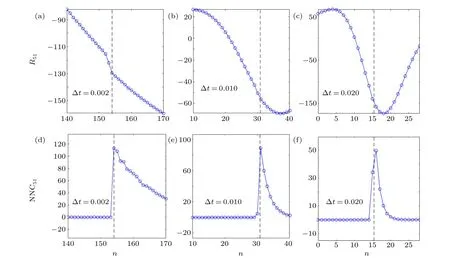
Fig.5. Comparison of our method and the FVN method[36] for the example of a linearly coupled Lorenz network as in Eq.(22). All the dashed lines represent the actual time delay nij,τij =nijΔt. (a)Δt=0.002 and the amount of data Ndata=109. (b)Δt=0.010 and Ndata=2×108. (c)Δt=0.010 and Ndata=108. (d)Δt=0.002. (e)Δt=0.010. (f)Δt=0.020. The number of resets M=5×104 in(d)-(f).

Fig.6. The numerical discrete delays ˆni1 and coupling coefficients ˆWi1 for the FVN method and our method(RSVR).Δt =0.002. (a)The numerical ˆni1 plotted against the actual ni1. (b)The numerical ˆWi1 plotted against the actual Wi1.

Both our method and the FVN[36]method can reconstruct time-delayed interactions of dynamic networks with noises,hidden variables and nodes. For these two methods,detection of the interaction between two nodes only needs the output of these two nodes, so network sizes and structures do not affect the calculated results significantly. Only average coupling strength can be inferred through the FVN method,[36]while our method can reconstruct the equivalent coupling function no matter whether it is linear as in Fig.1(d)or nonlinear as in Figs. 3(a) and 4(a). Moreover, our method has better robustness for sampling intervals.

Finally, we consider weak couplings. For a very weak coupling, ifWij →0, the equivalent coupling functionh′ij(xj,τij)→0 and ～hi j(xj,τ)→0 (Eq. (16)). According to Eq.(17),NNCij(τij)→0,and we cannot observe a significant increment for NNCij(τij).Thus we cannot identify actual time delayτij,and thenWijis also not available.

5. Conclusion

In this paper,we introduced a random state variable resetting method to detect the coupling functions of time-delayed dynamic networks. The nearest neighbor correlation function has been defined and calculated for measurable data by arbitrarily resetting the variable ofj. The time delay of nodejto nodeican be determined by utilizing the increment of the nearest neighbor correlation at the actual time delay. The error of a reconstructed time delay only depends on the sampling interval. Our proposed method has satisfactory reconstruction results for time delays even if the sampling interval is relatively large. Based on the determined time delays, the equivalent coupling functions can be estimated. Simulation results demonstrated that the random state variable resetting method and the nearest neighbor correlation function proposed can be used to detect the interactions of time-delayed dynamic networks.