Adaptive cubature Kalman filter based on variational Bayesian inference under measurement uncertainty①
2022-02-11HUZhentao胡振涛JIAHaoqianGONGDelong
HU Zhentao(胡振涛),JIA Haoqian,GONG Delong②
(*School of Artificial Intelligence,Henan University,Zhengzhou 450046,P.R.China)
(**Laboratory and Equipment Management Office,Henan University,Zhengzhou 450046,P.R.China)
Abstract
Key words:variational Bayesian inference,cubature Kalman filter(CKF),measurement uncertainty,Inverse-Wishart(IW)distribution
0 Introduction
Nonlinear dynamic system has been widely applied in many applications,such as rocket guidance,inertial navigation of aircrafts and ships,radar or sonar detection and target tracking[1].Recently,although extended Kalman filter has been applied in various fields,its inherent shortcomings also limit its development.Due to the use of linearization to approximate nonlinear function,the estimation accuracy is reduced,and the tedious Jacobian matrix needs to be calculated[2].Particle filter is a random sampling filter,which approximates the posterior mean of the state by a series of sampling points,and approximates the probability distribution function of the state by random particles.However,its estimation accuracy is excessively dependent on the number of sampling points[3].Sigmapoint Kalman filter includes filters such as unscented Kalman filter(UKF)and cubature Kalman filter(CKF).These filter algorithms are all based on certain sampling strategies to obtain the determined sampling points,and then these sampling points are used to calculate the approximate Gaussian integral.However,for high-dimensional nonlinear systems with higher vector dimensions,the covariance of UKF may be nonpositive in the filtering process,which results in unstable or even divergent filtering values[4].Compared with above algorithms,CKF has higher filtering accuracy,better numerical stability and lower computational complexity[5].
Due to the limitations of sensor performance and the surrounding environment,the infinite accurate measurement information cannot be obtained.Considering the influence of weather,humidity and other environmental factors may lead to time-varying measurement noise[6],Ref.[7]proposed the Sage-Husa adaptive filter(SHAKF)to solve the problem that the measurement noise is time-varying and the prior information such as its statistics is unknown.The filter recursively estimates the noise statistics based on the maximum a posteriori criterion to reduce the influence of noise on the estimation results.However,the use of SHAKF cannot guarantee the convergence to the correct noise covariance matrix,which may lead to filtering divergence.Ref.[8]realized the joint estimation of measured noise distribution parameters and system state in the state space model system under the variable Bayesian(VB)framework combined with inverse gamma distribution.However,the use of inverse gamma distribution leads to large amount of calculation and poor universality.Ref.[9]proposed an adaptive linear Kalman filter based on VB,which uses the Inverse-Wishart(IW)distribution as the conjugate prior distribution of the measurement noise covariance matrix,updates the approximate posterior distribution of the system state and noise parameters through the fixed-point iterative method.In addition to the time-varying noise,the hardware failure of the sensor will also cause the random measurement losses.The sensor only receives pure noise,which does not contain any useful information of the target[10].If the sensor knows whether the measurement is lost in advance,the minimum variance estimation(MVE)of the linear Gaussian system can be provided by the intermittent Kalman filter(IKF)[11].In reality,the sensor cannot predict whether the measurement information is lost.Ref.[12]proposed BKF-I and BKF-II based on the maximum a posteriori probability estimation criterion to solve the measurement losses,but they cannot adaptively estimate the measurement loss probability.Ref.[13]proposed a new VB-based adaptive Kalman filter(AKF)to solve the problem of unknown measurement loss probability,but this algorithm has not been extended to the nonlinear field.
In this paper,a new adaptive cubature Kalman filter based on variational Bayesian inference is proposed.Aiming at the problem of unknown measurement noise covariance matrix and measurement loss probability in measurement model,the conjugate prior distribution of unknown parameters and estimated state is established firstly,and then the posterior probability density function(PDF)of state,noise covariance matrix,decision factor and measurement loss probability are updated to Gaussian distribution,inverse Wishart distribution,Bernoulli distribution and Gamma distribution by variational Bayesian inference.Finally,the estimated variables can be obtained;at the end of the paper,the simulation results verify the effectiveness of the proposed VBACKF.
1 Problem description
Consider the following discrete-time non-linear stochastic system described by the state-space model.

wherexk∈Rnandzk∈Rmare the state vector and measurement,respectively;f(·)represents the nonlinear state transition function,h(·)represents the nonlinear observation function;wk∈Rnandvk∈Rmare respectively Gaussian process and measurement noise vectors with zero mean vectors and covariance matricesQkandRk.The initial state vectorx0∈Rnis assumed to have a Gaussian distribution with mean vector0|0and covariance matrixP0|0.ξkobeys a Bernoulli distribution with only two possible values:1 and 0.Obviously,ξk=1 represents the real measurement information obtained by the sensor at timek,andξk=0 represents the measurement lost at timek.The probabilities of the Bernoulli random variablesξktaking the values of 1 and 0 are given as

where,Pr(ξ)represents the probability ofξktaking 0 or 1,andτkrepresents the measurement loss probability at timek.Moreover,wk,vk,ξkandx0are assumed to be mutually uncorrelated for any time.
2 Methodology
2.1 The choice of prior distributions
One-step prediction probability density functionp(xk|z1:k-1)satisfies Gaussian distribution.

where,N(·;μ,Σ)denotes the Gaussian PDF with mean vectorμand covariance matrixΣ;k|k-1andPk|k-1are the one-step prediction state estimation atktime and the corresponding estimation error covariance matrix,respectively.At the same time,since the measurement noise covariance matrixRkis time-varying,it is necessary to find its posterior distribution,which requires selecting the appropriate conjugate prior distribution forRk,that is because the conjugate can ensure that the posterior distribution and the prior distribution have the same function form.In Bayesian statistics,IW distribution is usually chosen as the conjugate prior distribution of covariance matrix of Gaussian distribution with known mean[14].Therefore,IW distribution is selected as the prior distribution ofRk

where IW(Rk;k|k-1,k|k-1)denotes the IW distribution with degree of freedom parameterk|k-1and inverse scale matrixk|k-1.The probability density function of IW distribution can be expressed as
IW(A;u,U)=

whereAis the covariance matrix ofn-dimensional time-varying Gaussian vector,uis the degree of freedom parameter,Uis then-dimensional inverse scale matrix,tr(·)represents the trace of the matrix,and Γn(·)is ann-dimensional Gamma function.WhenA~IW(A;u,U)andu>n+1 are satisfied,E[A-1]=(u-n-1)U-1is established[15].
The prior parameters of predicting measurement noise are obtained by


Although the prior information of measurement noise is obtained,the random measurement losses will also reduce the estimation accuracy.It is necessary to estimate the probability of measurement losses,and then the measurement noise covariance matrix is modified.
The conditional likelihood probability density function in Eq.(2)can be expressed as
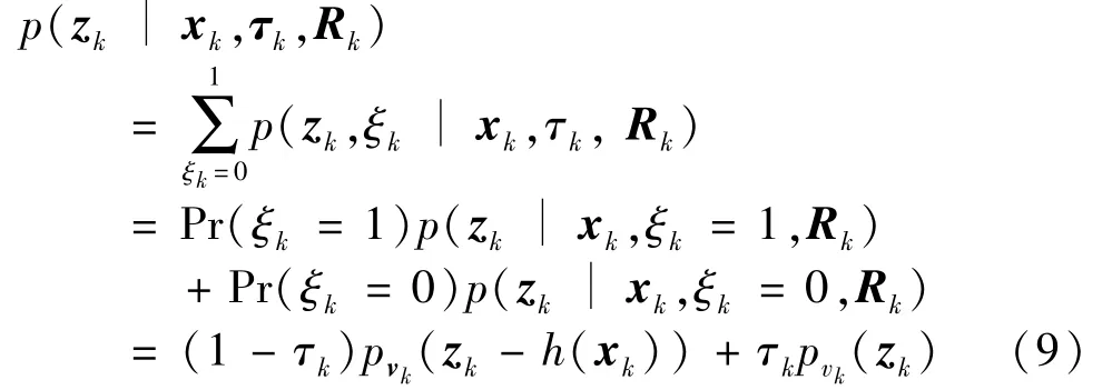
wherepvk(·)denotes the probability density function of measurement noise.Eq.(3)and Eq.(4)can be transformed into the following probability-mass function(PMF).

Combining Eq.(9)and Eq.(10),the likelihood probability density functionp(zk|xk,τk,Rk)can be rewritten as


So conditional likelihood probability density functionp(zk|xk,ξk,Rk)can be expressed as the following exponential multiplication form.

Further,the probability density functionp(zk|xk,ξk,Rk)can be rewritten as

In addition,zkdepends not only onxkandRk,but also onξkandτk,so it is necessary to calculate the joint prior probability density function.

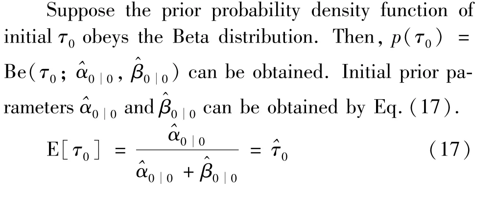
whereΞ≜{xk,ξk,τk,Rk}represents the set of estimated variables,p(τk|z1:k-1)represents the prior probability density function of the measurement loss probability at timek.The prior distributionp(τk|z1:k-1)is selected as a Beta PDF since the Beta distribution is a conjugate prior to the Bernoulli distribution,so that the prior distribution and posterior distribution ofτkhave the same form[16]:


here,η∈(0,1]denotes a forgetting factor used to spread the posterior PDFp(τk|z1:k-1).
2.2 The variational approximation of posterior probability density function
In order to estimatexktogether withξk,τkandRk,the joint posterior PDFp(xk,ξk,τk,Rk|z1:k)needs to be computed.Since the form of joint posterior probability density functionp(xk,ξk,τk,Rk|z1:k)is very complex and its analytical solution cannot be directly obtained.To make the joint posterior distribution easy to handle,the approximate free solution of joint posterior probability density function is obtained by VB method.Then,it can be obtained whereq(·)represents the variational approximate posterior probability density function ofp(·).

According to the VB approximation idea,the optimal approximation of the posterior probability density function of the estimated variable is obtained by minimizing the Kullback-Leibler divergence(KLD)between the factored approximate posterior PDFq(xk)q(ξk)q(τk)q(Rk)and true joint posterior PDFp(xk,ξk,τk,Rk|z1:k-1)


According to VB approach,the optimal solution of Eq.(19)satisfies the following equation.

where E[·]represents the expectation operation,and log(·)represents the logarithmic function.θis an arbitrary element ofΞ,Ξ(-θ)is the set of all elements inΞexcept forθ.cθrepresents the constant term related toθ.
According to Eq.(20),the expectation of logarithmic joint posterior probability density function is required to obtain the approximate posterior probability density function of the estimated variables.However,since the approximate posterior distributionq(xk),q(ξk),q(τk)andq(Rk)are coupled with each other,the analytical solution cannot be obtained directly by Eq.(20).Therefore,the fixed-point iteration method is adopted to solve this problem[9].
According to the conditional independence of the state space model,the joint probability density functionp(Ξ,z1:k)can be expressed as

Substituting Eq.(5),Eq.(6),Eq.(10),Eq.(13)and Eq.(15)into Eq.(21),Eq.(22)can be obtained

According to Eq.(22),logp(Ξ,z1:k)can be expressed as
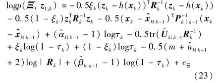
Letθ=Rkand substitute Eq.(23)into Eq.(20),logq(i+1)(Rk)can be written as given by

whereq(i+1)(·)represents theapproximated probability density functionofp(·)at the(i+1)th iteration.Ais given by

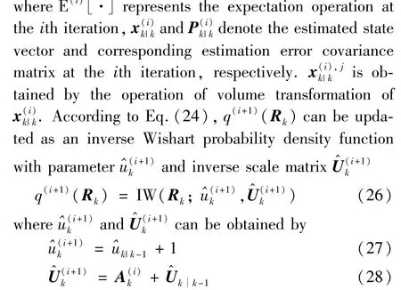
Letθ=xkand substitute Eq.(23)into Eq.(20),logq(i+1)(xk)can be written as given by

According to Eq.(29),q(i+1)(xk)can be updated as
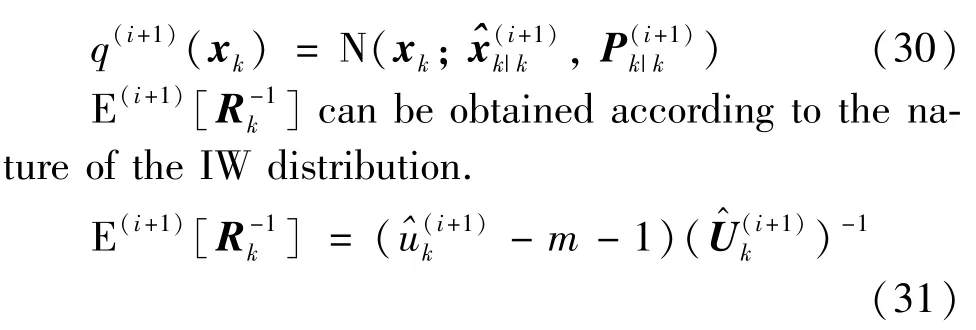
Exploiting Eq.(31),the modified measurement noise covariance matrixsatisfies

where E(i)[ξk]can be obtained through Eq.(42)at theith iteration.
Letθ=ξkand substitute Eq.(23)into Eq.(20),logq(i+1)(ξk)can be written as

According to Eq.(33),the posterior probability of the Bernoulli random variableξtaking the values of 1 and 0 are given by

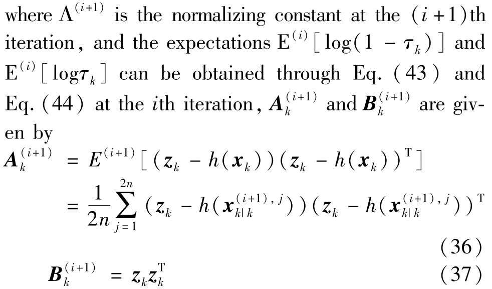
Letθ=τkand substitute Eq.(23)into Eq.(20),logq(i+1)(τk)can be written as

According to Eq.(38),q(i+1)(τk)can be updated as
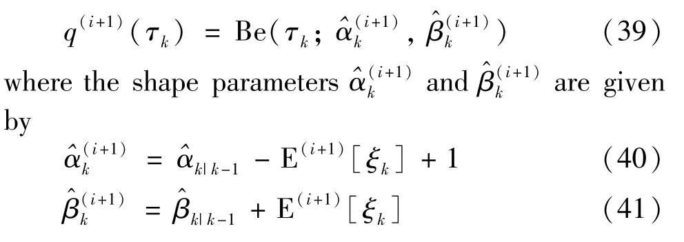
The expectations E(i+1)[ξk],E(i+1)[logτk]and E(i+1)[log(1-τk)]are given by
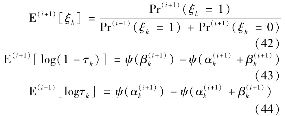
whereψ(·)is a Digamma function[17].
The implementation of VBCKF algorithm is as follows.
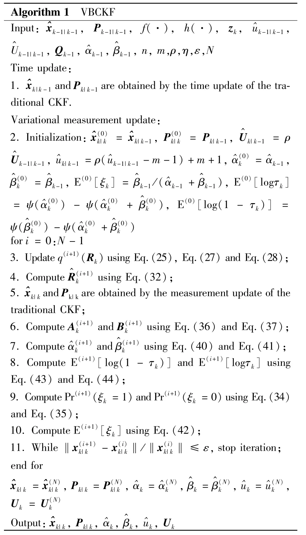
Algorithm 1 VBCKF Input:^xk-1|k-1,Pk-1|k-1,f(·),h(·),zk,^uk-1|k-1,U^k-1|k-1,Qk-1,^αk-1,β^k-1,n,m,ρ,η,ε,N Time update:1.^xk|k-1 and Pk|k-1 are obtained by the time update of the traditional CKF.Variational measurement update:2.Initialization:^x(0)k|k=^xk|k-1,P(0)k|k=Pk|k-1,U^k|k-1=ρ U^k-1|k-1,^uk|k-1=ρ(^uk-1|k-1-m-1)+m+1,^α(0)k=^αk-1,β^(0)k=β^k-1,E(0)[ξk]=β^k-1/(^αk-1+β^k-1),E(0)[logτk]=ψ(^α(0)k)-ψ(^α(0)k+β^(0)k),E(0)[log(1-τk)]=ψ(β^(0)k)-ψ(^α(0)k+β^(0)k)for i=0:N-1 3.Update q(i+1)(Rk)using Eq.(25),Eq.(27)and Eq.(28);4.Compute R^(i+1)k using Eq.(32);5.^xk|k and Pk|k are obtained by the measurement update of the traditional CKF;6.Compute A(i+1)k and B(i+1)k using Eq.(36)and Eq.(37);7.Compute^α(i+1)k andβ^(i+1)k using Eq.(40)and Eq.(41);8.Compute E(i+1)[log(1-τk)]and E(i+1)[logτk]using Eq.(43)and Eq.(44);9.Compute Pr(i+1)(ξk=1)and Pr(i+1)(ξk=0)using Eq.(34)and Eq.(35);10.Compute E(i+1)[ξk]using Eq.(42);11.While‖x(i+1)k|k-x(i)k|k‖/‖x(i)k|k‖≤ε,stop iteration;end for^xk|k=^x(N)k|k,Pk|k=P(N)k|k,^αk=^α(N)k,β^k=β^(N)k,^uk=^u(N)k,Uk=U(N)k Output:^xk|k,Pk|k,^αk,β^k,^uk,Uk
3 Simulation results and analysis
The simulation experiment scene is set as a typical two-dimensional plane target tracking.The proposed VBACKF is compared with cubature Kalman filter(CKF)[5],variational Bayesian cubature Kalman filter(VBCKF)[9],Bayesian cubature Kalman filter(BCKF1)[12],posterior distribution Bayesian cubature Kalman filter(BCKF2)[12],adaptive cubature Kalman filter(ACKF)[13]and intermittent cubature Kalman filter(ICKF)[11].In the above algorithms,ICKF is used as the standard algorithm,because it has the best filtering accuracy with the correct measurement statistics.The feasibility and effectiveness of the proposed VBACKF are verified by comparing multiple metrics.
3.1 Simulation model and parameters

The state equation and measurement equation in the target tracking model are given as wherexk=[xk,̇xk,yk,̇yk]Tis the state vector,xkanḋxkrepresents the position and velocity of the target in the horizontal direction at timek,respectively;ykanḋykrepresents the position and velocity of the target in the vertical direction at timek,respectively;ωis the turn rate;Tis the sampling interval;wk-1is the zeromean Gaussian process noise vector and its covariance matrixQk=diag[qM qM],qis the scalar parameter,Mis given by

The measurement noisy vectorvkis time-varying,and its covariance matrix changes as

whereR'k=diag[1020.1],tsis the total steps of a certain Monte Carlo run.
The number of Monte Carlo runsM,the number of iterationsNmand other simulation experiment parameters are given in Table 1.
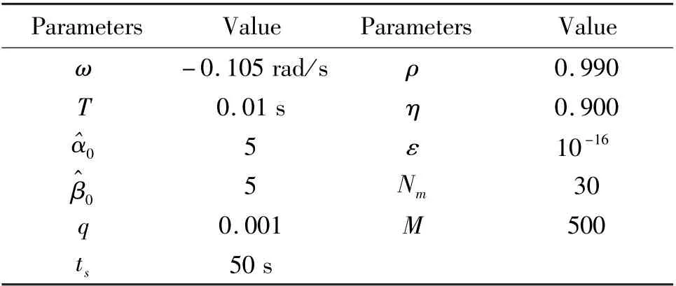
Table 1 Simulation parameters
3.2 Performance metrics
The root-mean square error(RMSE)and the averaged root-mean square error(ARMSE)of the position are chosen as the performance metrics to evaluate the accuracy of all algorithms,their definitions are as follows.
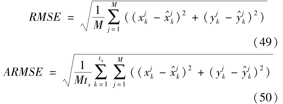
In order to evaluate the estimation accuracy of measurement noise covariance matrix,the square root of normalized Frobenius norm is selected as the performance metrics.

where‖X‖2=tr(XXT),andrepresent the estimated measurement noise covariance matrix and the real measurement noise covariance matrix at timekin thejth Monte Carlo run,respectively.
3.3 Simulation results and analysis
Two scenarios are designed to test the performance of the filter,which are scenario 1 with constant measurement loss probability(P(τk)=0.1)and scenario 2 with time-varying measurement loss probability.The measurement loss probability in scenario 2 changes as follows.

Fig.1 and Fig.2 show the RMSEs estimated by seven filtering algorithms in two different scenarios.Fig.3 and Fig.4 show the measurement loss probability estimated by ACKF and VBACKF in two different scenarios.
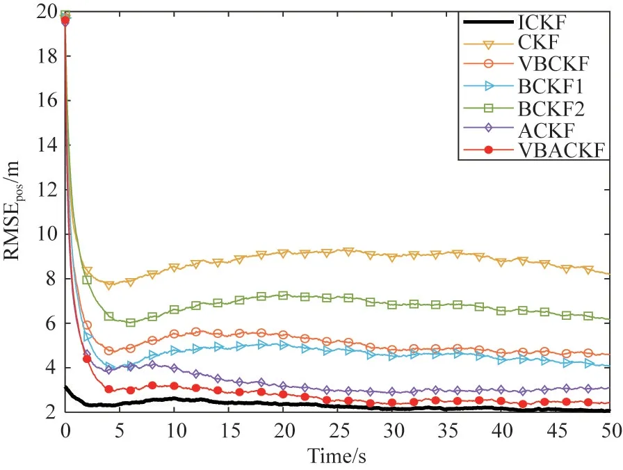
Fig.1 RMSEs of different filters(scenario 1)
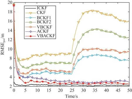
Fig.2 RMSEs of different filters(scenario 2)
In order to more intuitively compare the estimation accuracy of all algorithms,Table 2 shows the ARMSE from 5 s to 50 s estimated by seven filtering algorithms in two scenarios.
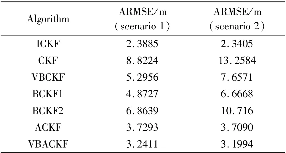
Table 2 ARMSE of position estimation
Through Table 2,it can be seen that the ARMSE of VBACKF is 38.80% higher than that of VBCKF.This is because VBCKF cannot process random measurement losses,which results in low filtering accuracy.In addition,the estimation accuracy of BCKF1 and BCKF2 is 33.48% and 52.80% lower than that of VBACKF,respectively.The reason is that the two filters rely on the correct prior information.When they cannot obtain accurate measurement loss prior information,the estimation accuracy will decrease significantly.However,the VBACKF algorithm proposed in this paper can adaptively estimate the measurement loss probability,as shown in Fig.3 and Fig.4.The estimation accuracy of VBACKF is 13.10% higher than that of ACKF.As shown in Fig.5,the measurement noise used by VBACKF is closer to the real measurement noise.This is because ACKF cannot solve the problem of time-varying measurement noise.In addition,the use of measurement noise covariance with too large deviation will also lead to inaccurate corrected measurement noise covariance,which will reduce the accuracy of the algorithm to estimate the measurement loss probability,as shown in Fig.3 and Fig.4.
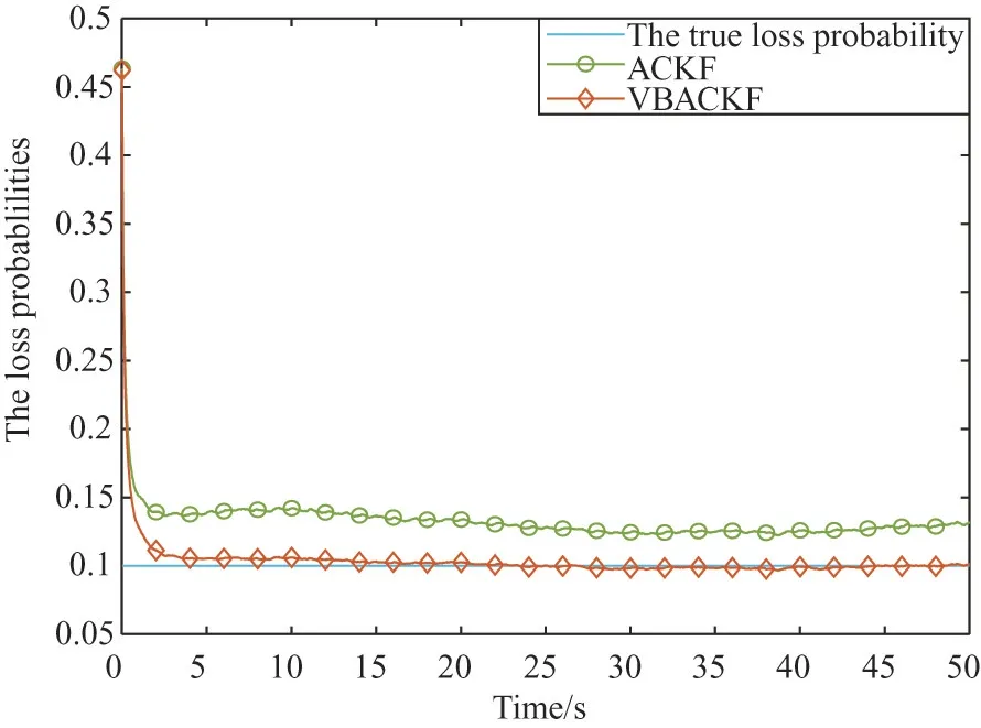
Fig.3 Measurement loss probability estimation(scenario 1)
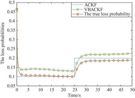
Fig.4 Measurement loss probability estimation(scenario 2)
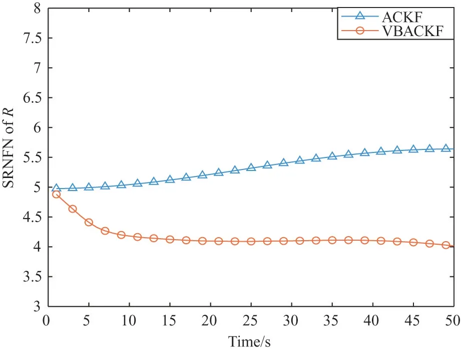
Fig.5 SRNFN of measurement noise covariance matrix
Fig.6 and Fig.7 show the real measurement losses and estimated measurement losses of 50 steps in a single Monte Carlo simulation under the scenarios with measurement loss probabilities of 0.1 and 0.2,respectively.The circle indicates the true measurement losses,and the dot indicates the estimated measurement losses.When the circle and the dot coincide,the judgment is correct.The diagram shows that the proposed VBACKF filter can accurately judge whether the measurement is lost.
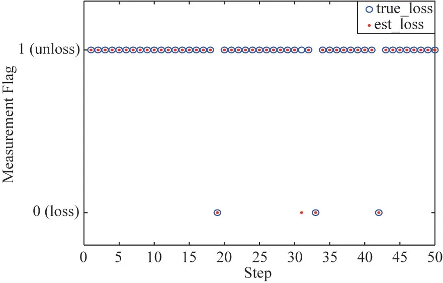
Fig.6 Measurement loss of truth and judgment(τk=0.1)

Fig.7 Measurement loss of truth and judgment(τk=0.2)
Fig.8 shows the influence of different sensor measurement loss probability on VBACKF position estimation.The figure shows that when the sensor measurement loss probability increases from 0.1 to 0.5,the RMSE increases slowly.The reason is that the proposed algorithm can estimate the measurement loss probability in real time,and further modifies the measurement noise covariance according to the estimation results.However,the measurement loss probability of the sensor gradually increases to 0.5,the RMSE value increases significantly,which is because the measurement loss occurs more frequently.As shown in Fig.9,when the loss probability increases from 0.5 to 0.9,the detection success rate of VBACKF decreases sharply,meanwhile resulting in a significant decrease in the estimation accuracy.

Fig.8 RMSE of position target estimation under different loss probabilities

Fig.9 Success rate of VBACKF detection under different loss measurement probability
4 Conclusions
A novel variational Bayesian inference based on adaptive cubature Kalman filter(CKF)is proposed to improve the influence of unknown measurement noise covariance and measurement loss probability on estimation accuracy.In the CKF framework,the VB method is introduced,and the IW distribution is selected as the conjugate prior distribution of the measurement noise covariance matrix.The beta distribution is selected to model the measurement loss probability density function.The fixed-point iteration method is used to iteratively solve the posterior distribution of the coupling estimated variables.The proposed VBACKF has higher estimation accuracy,adaptability and robustness than traditional filtering algorithms.It can be further extended to group target tracking and extended target tracking.
杂志排行
High Technology Letters的其它文章
- Design and implementation of near-memory computing array architecture based on shared buffer①
- Design and experimental study of active balancing actuator driven by ultrasonic motor①
- Trajectory tracking control of characteristic model for nonplanar hex-rotor UAV①
- The adaptive distributed learning based on homomorphic encryption and blockchain①
- HOPE:a heterogeneity-oriented parallel execution engine for inference on mobiles①
- Joint utility optimization algorithm for secure hybrid spectrum sharing①
