Does Environmental Regulation Increase Employment? Based on the SCM and RCM Methods

Guo Lin and Zhang Xufei

Zhejiang University

Abstract: Whether environmental regulation can increase employment is still controversial in academic circles around the world. An important reason lies in the validity of an empirical method. Using China’s inter-provincial panel data from 2003 to 2015 and the synthetic control method (SCM), this paper focuses on a test that was carried out on the basis of a quasinatural experiment of the 2007 Emission Trading Pilot (ETP) policy. The test results show that the ETP policy has increased the average employment level by 3.25 percentage points and passed a robustness test. The robustness test using the regression control method (RCM) shows that the average employment level has risen by 3.21 percentage points. This means that the ETP policy has significantly increased employment. The paper also puts forward three policy recommendations: optimizing the trading system for emissions rights, encouraging companies to carry out cleaner production and innovation, and incorporating environmental performance assessments.

Keywords: environmental regulation, employment, synthetic control method, regression control method

Introduction

China’s 2020 Report On The Work Of The Government pointed out that “we will strive to keep existing jobs secure, work actively to create new ones, and help unemployed people find work,” and also “we will endeavor to protect our blue skies, clear waters, and clean lands, and meet the goals for the critical battle of pollution prevention and control.” These objectives indicate the central government’s focus on environmental protection and employment issues. This is closely related not only to the harmonious coexistence of man and nature but also to people’s work and life. Theoretically, when a government strengthens its supervision over environmental protection, it will also generate additional costs for emission reduction to enterprises and thus reduce their profits and decrease the scale of labor employment. In this case, environmental regulatory policies may have a negative effect on employment. A question therefore arises: Do environmental regulation and employment development conflict with each other? If the two strategies really cannot coexist in harmony, then the policy effect will be dramatically reduced. In order to solve this problem, a key breakthrough is to delve into the potential causal relationship between the two, which can provide some guidance for policy formulation and rational expectation for the effect of policy implementation.

Previous academic research has studied the relationship between environmental regulatory policies and employment, but opinions on the specific relations between them are quite different. These opinions can roughly be divided into three types: The first type believes that environmental regulatory policies can promote employment (Carraro, Galeotti & Gallo, 1996; Golombek & Raknerud, 1997; Marx, 2000; Morgenstern, Pizer & Shih, 2002; Gray, Shadbegian & Wang, 2013; Chen, 2011; Hafstead & Williams, 2016; Sun & Zhou, 2019); the second type holds that environmental regulatory policies would inhibit employment (Hartman, 1979; Henderson, 1997; Greenstone, 2002; Bezdek & Wendling, 2008; Jiang, 2017; Yan & Guo, 2017); the third type believes that environmental regulatory policies and employment have a non-linear or irrelevant relationship (Goodstein, 1994; Rolf & Arvid, 1997; Berman & Bui, 2001; Lu, 2011; Kahn & Mansur, 2013; Li, 2015; Lou & Ran, 2016; Li, 2016; Qin, Liu & Sun, 2018). The difference is mainly due to the following two reasons: First, the theoretical mechanism is uncertain. Generally speaking, environmental regulatory policies exert scale and substitution effects on employment (Berman & Bui, 2001; Lu, 2011; Li, 2015; Li, 2016), and the two effects are usually opposite. The scale effect means that environmental regulation would increase the production costs of enterprises and reduce their competitive advantages. Then enterprises will reduce their scale and cause employment reduction. The substitution effect means that environmental regulation would increase the prices of resources, and enterprises then have to hire relatively cheap labor, which causes employment to rise. Second, the empirical method is biased. Most of the previous studies use ordinary regression methods, but Berman and Bui (2001) pointed out that it is difficult to estimate the effects of environmental regulation through regression methods because problems such as selection bias and measurement errors may arise in this process. For companies that can achieve emissions reductions at a small cost, environmental policies would have the least impact on their employment decisions, and such companies are most likely to reduce emissions voluntarily (even if they are not offered regulatory incentives). The effect of this choice will make the cost of pollution abatement lower than it actually is. Besides, due to measurement bias, measurement errors in abatement costs are likely to deflect the estimated effect toward zero.

In 2007, China implemented the largest sulfur dioxide ETP policy in 11 provinces, which is equivalent to an unusual “quasi-natural experiment.” To further identify the causal relationship between environmental regulatory policies and employment, the ETP policy provides a valuable opportunity. Yan and Guo (2017) used the Difference in Difference (DID) method to explore the impact on environmental regulatory policies. The study found that the ETP policy did not bring out a double dividend effect of the environment and employment. Different from their empirical methods, this paper uses the SCM to re-examine the causal relationship between environmental regulatory policies and employment for two main reasons: First, Su and Hu (2015) pointed out that the DID method can overcome the problem of selection bias in a better way, but the progress and intensity of policy implementation in each province after 2007 are so different that using the control group to reflect the policy effectiveness is not accurate enough; Second, SCM is a data-driven method which synthesizes the control group to provide a total contribution and each individual’s sub-contributions and thus can effectively avoid averaging and excessive extrapolation. On the other hand, Hsiao et al. (2012) proposed using the regressive control method (RCM), which is very similar to SCM. The main difference is that RCM allows the weight of the control group to be negative. This can avoid the impossibility of finding a suitable control group to simulate the situation of the treated group (Wu & Xie, 2019). Based on this consideration, this paper uses RCM for a robustness test. Specifically, the main contributions of this paper include: First, it is the first time that SCM has been used to accurately measure the marginal dynamic impact of the ETP policy on employment to make up for the gap of the current empirical research methods; Second, it is the first time that RCM has been used for a supplementary test to increase the validity of empirical results; Third, the research results of this paper provide empirical evidence and decision-making support for balancing environmental regulation and employment development.

This paper is structured as follows: The second part presents a literature review and policy background; the third part focuses on the research design, covering details such as mathematical models, data sources, variable interpretations, and balance tests; the fourth part shows empirical analysis, including basic analysis, robust analysis, and a placebo test; the fifth part describes a further test with RCM; the last part covers conclusion and policy recommendations.

Literature Review and Policy Background

Literature Review

Previous studies on environmental regulation and employment can mainly be divided into three branches: The first branch believes that environmental regulation promotes employment development. Carraro et al. (1996) used a general equilibrium model to simulate the taxation effect of European carbon taxes, and the results showed that the levy of carbon taxes could produce a double dividend effect on employment in the short term. Golombek & Raknerud (1997) found that environmental regulation could positively promote labor employment in steel and manufacturing industries. Marx (2000) believed that there is a complementary relationship between environmental protection and employment. He found that environmental protection could create jobs, yet it may reduce employment in some other industries, but the net effect between them was positive. Morgenstern et al. (2002) and Gray et al. (2013) conducted empirical tests to analyze the relationship between environmental regulation and employment. They found that environmental regulation did not pose an obvious negative effect on employment, and in some fields, it even exerts a positive promoting effect. Chen (2011) used the panel data of China’s industrial sector from 2001 to 2007 for her study and found that environmental regulation can promote employment. Hafstead & Williams (2016) believed that the collection of pollution taxes had a positive effect on employment in industries that were less pollutionintensive. Sun & Zhou (2019) analyzed the impact of environmental regulation on employment structure using inter-provincial panel data from 2006 to 2016 and found that the implementation of environmental regulations had a significant positive role in promoting employment upgrading in the region.

The second branch believes that environmental regulation inhibits employment development. Hartman (1979) found that federal environmental regulation reduced employment in the copper industry in the US. Henderson (1997) and Greenstone (2002) believed that environmental regulation would increase production costs of enterprises, then weaken their competitive advantages and reduce their scale of production, leading to a decrease in employment. Therefore, they hold that environmental regulation and employment contradict each other. Bezdek & Wendling (2008) studied the scale of the environmental protection industry in the US and employment related to the industry and found that environmental regulation had increased the prices of resource production factors, making companies more inclined to use labor as a substitute. Therefore, they hold that increasing investment in the industry would be conducive to promoting employment growth. Jiang (2017) used China’s provincial panel data from 2000 to 2014 and the spatial Durbin model to examine the relationship between China’s environmental regulation and employment. From a qualitative point of view, he found that environmental regulation in eastern China had promoted employment while that in its central and western regions had inhibited employment. Yan & Guo (2017) used China’s 2005-2012 corporate data and the DID method to test employment effects and found that the ETP policy had significantly reduced the employment scale of high-sulfur-emission or high-polluting companies. Subsequently, he used a platform-specific model (PSM) in combination with the DID method to make further analysis.

The third branch believes that environmental regulation and employment are irrelevant or have a non-linear relationship. Goodstein (1994) analyzed a questionnaire on the cause of unemployment provided by the US Department of Labor and found that the impact of environmental policies on unemployment in the country from 1987 to 1990 was only 0.1 percent, which meant that only 500 people out of the 500,000 unemployed were due to environmental regulation. Rolf & Arvid (1997) believe that environmental regulation had a negative scale effect and an uncertain substitution effect on employment, so the overall employment effect was uncertain. Berman & Bui (2001) directly used control measures and factory data to estimate the impact of the dramatic increase in air quality control in Los Angeles on employment. They found no evidence that local air quality control had greatly reduced employment. Lu (2011) simulated the double dividend effect of China’s employment on the basis of a Value at Risk (VaR) model and finally found that a carbon tax of RMB10 per/ton had no significant impact on employment. He concluded that, at least so far, it has been difficult for China to obtain the double employment bonus in the short term. Kahn & Mansur (2013) believed that differences in environmental regulatory standards in different regions had caused the spatial transfer of employment, and the flow of labor in areas meeting environmental standards and those that did not meet environmental standards had an uncertain impact on employment. Li (2015) drew on the method of introducing environmental pollution intensity to an AK model and derived a model of influencing factors of employment through producer equilibrium conditions. Then she used China’s provincial dynamic panel data from 1995 to 2012 to empirically test the relationship between environmental regulation and employment. She found that there was a U-curve relationship between environmental regulation and employment. Considering the heterogeneity of regional income and education levels, the relationship between environmental regulation and employment was complex and diversified. Lou & Ran (2016) found that environmental regulation and employment had a negative linkage effect in some industries of the primary and secondary sectors and a positive linkage effect in other industries of the secondary sector and the tertiary sector. Li (2016) analyzed the scale, substitution, and pollution emission reduction effects of environmental regulation on the labor demands of enterprises based on a partial equilibrium model of production and then conducted an empirical test using panel data from China’s industrial sectors. He found that environmental regulation had a U-shaped relationship with total employment. According to his research, with the enhancement of environmental regulation, its impact on employment had turned from negative to positive. Based on an improved entropy method, Qin et al. (2018) tested the industry heterogeneity impact of environmental regulation on employment using 37 industry-specific panel data from 2007 to 2014. They found that there was a U-shaped relationship between the two in industries with heavy pollution. In industries with slight or medium pollution, there was an inverted U-shaped relationship between the two. An increase in the share of labor costs and a decrease in industry monopoly would weaken the employment elasticity caused by environmental regulation.

Policy Background

Emissions trading originated in the US. The American economist John H. Dales was the first one to propose the theory of emissions trading in 1968. The gestation of the emission trading system in China can be traced back to the pilot emission permit system introduced in 1988. In 1993, Ministry of Ecology and Environment of the People’s Republic of China (formerly the National Environmental Protection Agency of China) began to explore the implementation of air pollution rights trading policies and designated Taiyuan, Baotou, and some other cities as the places for such pilot projects. In 1999, Ministry of Ecology and Environment of China and the US Environmental Protection Agency signed an agreement to set Nantong and Benxi cities as the earliest pilot bases to carry out a cooperative project in China named Research on Using Market Mechanisms to Reduce Sulfur Dioxide Emissions. In April 2001, Ministry of Ecology and Environment of the China and the US Environmental Protection Agency entered into an agreement concerning the Research on Promoting China’s Total Sulfur Dioxide Emission Control and the Implementation of Emission Trading Policies. Subsequently, in 2001, Nantong Tianshenggang Power Generation Co., Ltd. and another large chemical company in the city carried out sulfur dioxide emission rights trading, which was the first case of such trading in China. In March 2002, State Environmental Protection Administration (SEPA) and the US Environmental Protection Association jointly launched a research project to promote the implementation of China’s total sulfur dioxide emission control and emission trading policy (referred to as the “4+3+1” Project). The project was implemented in Shandong, Shanxi, Jiangsu, and Henan provinces, Shanghai and Tianjin municipalities as well as the city of Liuzhou, and China Huaneng Group Co., Ltd.. In 2003, Jiangsu Taicang Port Environmental Power Generation Co., Ltd. and Nanjing Xiaguan Power Plant reached an off-site transaction of SO2emission rights, setting a precedent for cross-regional transactions in China. Since 2007, Ministry of Finance of the P.R.C, the Ministry of Ecology and Environment of the P.R.C, and the National Development and Reform Commission (NDRC) approved eight provinces, including Jiangsu, Zhejiang, Hubei, Hunan, Shanxi, Shaanxi, Hebei, and Henan, two municipalities (Tianjin and Chongqing), and one autonomous region (Inner Mongolia) to carry out emission trading pilot projects. On November 10, 2007, the first domestic emissions trading center was established in Jiaxing city of Zhejiang province, marking the gradual institutionalization, standardization, and internationalization of emissions trading in China.

Research Design

The SCM Model

According to the ideas of Abadie and Gardeazabal (2003), Abadie and Diamond (2010), and Wang and Nie (2010), only one region can be used as the treated group in SCM. In 2007, there were 11 provinces where ETP policy reforms were conducted. In order to use the SCM, this paper merges the 11 provinces to form a treated group in the first step and then synthesizes the remaining 20 provinces and cities to form a control group. The SCM is applied by the following steps:

First, we assume that the employment situation in M+1 regions is observed. The region in the first step (hereinafter referred to as “the first region”) is affected by the ETP policy. Then the remaining M regions are naturally treated as the control group. T0is used to represent the year of implementation of the ETP policy in 2007, and the total observation period is T, so 1 ＜ T0＜T naturally. According to the framework of a counterfactual state, we useto represent the employment status of regioninot to be tested in periodt, and useto represent the employment status of regionito be tested in periodt. Therefore, the employment impact of the ETP policy will be represented by. Assuming that before the start of the ETP policy, the employment levels in the pilot and non-pilot regions are the same, which means that fort≤ T0, we haveand when T0≤t≤ T, we have.

Then we useDitas a dummy variable for deciding whether it is affected by the ETP policy. If the areaiis affected by the policy during periodt, it is assigned a value of 1. Otherwise, it is 0. Then the result of the areaithat we have observed during periodtis. Before the implementation of the ETP policy, the employment in the treated area was the same as that in the non-treated area, so our goal is to estimate the employment change in the first region after the implementation of the ETP policy, which is. In this formula,Eitrepresents the employment situation of the treated area that has been observed over the past years.is the employment situation when the treated area is not affected by the ETP policy and which cannot be observed and needs to be estimated. We assume thatis determined by the following model:

In the above model,δtrepresents the time-fixed effect andzirepresents the observable variable that is not affected by the ETP policy, a (r×1) dimensional vector.θtis an unknown (1×r) dimensional parameter vector andλtis a common factor not observed in the (1×F) dimension.μtis the (F×1) dimension individual fixed effect whileεitis the error term with 0 as the average value. It is easy to find that this model is an extended version of the fixed-effect double-difference model.λtallows individual fixed effects to change over time, but if they do not change over time, the model will degenerate into a traditional double difference model. At the same time, associations betweenzi,μi, andεitare allowed.

In order to estimate the impact of the ETP policy, we must estimate the employment situationwhen the test area (the first region) is not affected by the policy. We can use other M (non-treated areas) to simulate the treated area without being affected by the ETP policy. To this end, we consider a (M×1)-dimensional weight vector W, which satisfiesωi≥ 0 for anyi, andω2+ … +ωM+1= 1. The vector W represents the combined weight of the remaining M regions to the first region (treated area).

Therefore, the result variable of synthetic control using W as the weight is:

Suppose there is a vector groupsatisfying:

Abadie et al. (2009) concluded that under normal conditions, the right side of the above formula will approach zero. Therefore, we can useas the unbiased estimate of, andcan further be used as the unbiased estimator of. In order to estimate, we need to know. In order for Equation (2) to be true, the eigenvectors of the first region need to be within the convex combination of the eigenvectors of other regions. Since exact solutions may not exist in practice, we need to estimate the approximate solution of. This paper chooses to minimize the distancebetweenX1andX0Wto determine the weight vector. Here W satisfies that for anym= 2,3, ..., M+1, there will beωi≥ 0 andω2+ … +ωM+1= 1.X1is the (k×1) dimensional feature vector of the test area before the ETP policy implementation whileX0is the (k×M) matrix. Column m ofX0is the corresponding eigenvector of the regionmbefore the ETP policy implementation, and the eigenvector is the factor or any linear combination that determines the employment situation in Equation (2). Generally speaking, in the distance function,Vis a (k×k) symmetric semi-definite matrix, and the choice ofVwill affect the estimated mean square error.

Referring to the practice of Abadie and Gardeazabal (2003), we also chose a symmetric positive semi-definite matrixVto minimize the mean square error of the employment estimation before the ETP policy implementation so that the employment situation in the composite area before the implementation is as close as possible to that in the treated area. It is worth mentioning that we require that the weight vector be non-negative so that the synthetic group is limited to the convex combination of the control group. The advantage of this approach is that it can reduce the bias of extrapolation due to the large difference between the control group and the treated group (King & Zheng, 2006). This paper uses the Synth package developed by Abadie to perform the model estimation.

Data Sources and Variable Explanation

This paper uses the provincial panel data from 2003 to 2015, which is obtained from theChinaStatistical Yearbookpublished by the National Bureau of Statistics, the statistical bureaus of provinces and cities, China Stock Market Accounting Research Database (CSMAR), and some other sources. The explained variable in this paper is the number of employees (Employ), which is measured by the number of employees in each province at the end of each year concerned. For the setting of the predictor variables, a reference was made to existing literature (Li, 2015; Li, 2016; Jiang, 2017; Qin et al., 2018; Sun & Zhou, 2019). Such variables include the consumer price index (CPI), an education level (School), R&D level (Author), capital deepening (Capital), nominal wage (Wage), economic development level (GDP), foreign direct investment (FDI), and industrial structure (Struc). In order to eliminate the influence of outliers, this paper performs a 1 percent shrinking treatment uniformly on all continuous variables. The main variables, meanings, and measurements applied in this paper are shown in Table 1:

Table 1 Variables

The Weight of Provinces in the Control Group

According to Abadie’s SCM model, the treated group can only involve one province, while the ETP policy pilot area mentioned in this paper consists of 11 provinces. Therefore, before conducting further analysis, we first summed up the corresponding variables of the 11 provinces each year and averaged them. In this way, a new treated group was formed. By then, our sample had changed from 31 to 21 provinces. Next, we used the SCM to select the optimal combination from the 20 provinces in the control group to synthesize the counterfactual situation of the treated group. Table 2 shows the weights of the 20 provinces. It can be seen that only six provinces have positive weights. The highest weight is Shandong province, with a weight value of 0.264, and the lowest weight is Tibet autonomous region, with a weight value of 0.029. This shows that the six provinces can achieve the best-fit effect, and therefore the remaining 14 provinces were no longer considered for the synthesis.

Table 2 The Weights of the Control Group

Province/Municipality/Autonomous Region Code Weight Shandong 8 0.264 Gansu 14 0.074 Other provinces e.g., 2 3 4… 0.000

Predictor Balance Test

Table 3 shows the comparison of the predictor variables of the treated group and the synthetic group before the implementation of the ETP policy in 2007. It can be seen that the gap is very small between the actual value and the synthetic value of all the predictor variables. The value of the maximum gap is only 0.3931, which shows that the synthetic group and the treated group have high similarity in economic characteristics, so the synthetic group can reflect to a large extent the counterfactual state of the treated group after the policy implementation.

Table 3 The Predictor Balance Test

Empirical Analysis

Basic Results

According to the weight of each province shown above, the synthetic group is constructed using the SCM. The top graph in Fig.1 shows the trend of employment changes between the treated group and the synthetic group over time. It can be seen that before the implementation of the ETP policy in 2007, the employment of the treated group and that of the synthetic group basically overlapped, indicating that the two groups had good comparability. It also means that the synthetic group can better fit the counterfactual situation of the treated group after the ETP policy implementation. After 2007, the employment of the synthetic group continued to maintain a stable rise while that of the treated group showed an obvious ascending trend and some fluctuations. This indicates that the ETP policy has significantly promoted employment. The bottom graph in Fig.1 shows the dynamic change in the employment gap between the synthetic group and the treated group, which reflects more inherently the net employment effect of the ETP policy implementation each year. Before 2007, the net employment effect is basically zero. After 2007, the net employment effect is obviously positive. Although the net employment effect decreases from 2008 to 2012, it is still obviously positive. After 2012, it increases significantly. In summary, the ETP policy has played a significant role in promoting employment.

Fig.1 Trend and Gap of Employment of the Two Groups from 2002 to 2016

Table 4 shows the accurate measurements of the employment of the treated group and the synthetic group each year. Before the implementation of the ETP policy in 2007, the employment of the treated group and that of the synthetic group were very close, with an average gap of only 0.0005, which indicates that the fitting effect is good. After the implementation of the ETP policy in 2007, the average gap between the two groups is 0.0325, indicating that the ETP policy has increased the employment level by an average of 3.25 percentage points.

Table 4 The Employment of the Two Groups

The Robustness Test

For Test 1, we used the number of patent applications to re-measure the level of R&D and the nested process to re-determine the weight of provinces, which is more accurate and robust than the default data-driven method. The specific empirical results are as follows: The top graph in Fig.2 shows that before the ETP policy implementation in 2007, the employment of the treated group and that of the synthetic group basically overlapped, indicating that the fitting effect is good. After 2007, the employment level of the treated group increased significantly. The bottom graph in Fig.2 shows the dynamic trend of the employment gap between the two groups each year vividly, reflecting the net employment effect of the policy implementation. Before 2007, the net employment effect is around 0. After 2007, the net employment effect is significantly higher. Although there are large fluctuations, the values remain significantly positive, indicating that the basic results are relatively robust.

For Test 2, we took into consideration the financial crisis in 2008, the implementation of the value-added tax (VaT) reform in 2009, and the pilot VaT reform in 2012 as these major exogenous events may have a great impact on employment after the ETP policy implementation. In order to eliminate the exogenous impact, we excluded all samples after 2008 and retested them. It can be seen from Fig.3 that before 2007, the employment of the treated group and that of the synthetic group basically overlapped while after 2007, the employment of the treated group increases significantly, showing that the basic results remain robust.

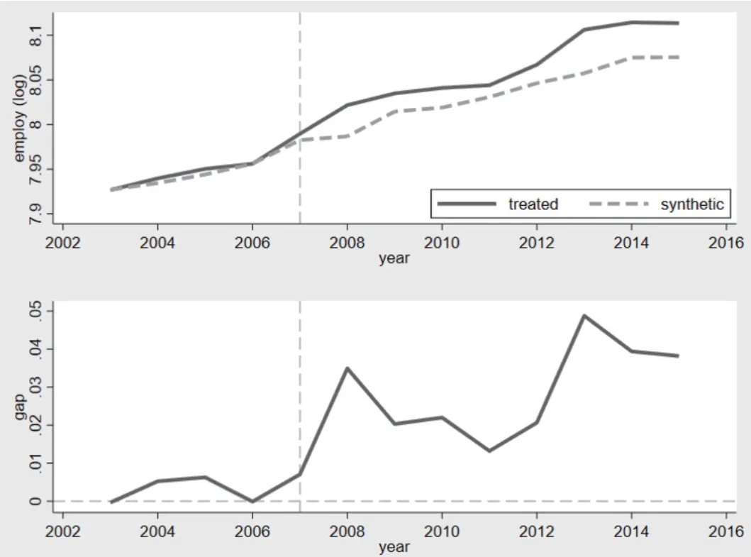
Fig.2 Trend and Gap of Employment of the Two Groups from 2002 to 2016

Fig.3 Trend and Gap of Employment of the Two Groups from 2002 to 2009

The Placebo Test

For Test 1, we used root mean square prediction error (RMSPE) to perform a placebo test. The specific calculation method is shown in the following formulas (5) and (6). The steps are as follows:

Firstly, we assume that the ETP policy has been implemented in any of the 21 provinces. The remaining 20 provinces are used as the control group. Secondly, we loop through the above process and get the time series of the fitting differences between the treated group and the synthetic group. Thirdly, we calculate the RMSPE before the ETP policy (Pre_RMSPE) and after the ETP policy (Post_RMSPE) separately and get the ratio (Post_RMSPE / Pre_RMSPE).

The concept of this method lies in that if the ETP policy is effective in the real treated group, the Post_RMPSE of the real treated group will be relatively large and the Pre_RMPSE relatively small. Therefore, it is expected that the RMPSE ratio of the real treated group should be relatively larger. The results are shown in Fig.4. It can be seen that the RMSPE ratio of the real treated group ranks second among 21 provinces with a statistical significance of 9.5 percent (0.095=2/ 21), indicating that the ETP policy has significantly promoted employment and passed the placebo test.

For Test 2, it is also assumed that the ETP policy has been implemented in any of the 21 provinces, and then the remaining 20 provinces are used as the control group. We repeat regressions to obtain 21 dynamic trend curves of the employment gap. It can be expected that the dynamic trend curve of the real treated group should be relatively larger. The result is shown in Fig.6. It can be seen from the left graph in Fig.5 that the dynamic trend curve (in bold) of the real treated group is not prominent among all the 21 curves. This does not seem to be in line with our expectations. Then what is the reason behind this result?

Fig.4 RMSPE Ratios of the 21 Provinces

Observing all the curves before the ETP policy implementation, we found that some of the curves fluctuate greatly and deviate significantly from the 0 value, indicating that their Pre_RMSPE values are high and their impacts are not credible. With reference to the practices of previous relevant studies, we eliminated the curves which are more than five times the Pre_RMSPE of the real treated group before the ETP policy implementation and finally retained nine provinces. The results are shown in the right graph in Fig.5. It can be seen that the curve of the real treated group (in bold) is quite prominent, indicating that the ETP policy has significantly promoted employment and passed the placebo test.

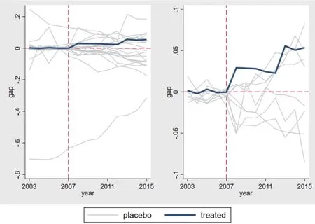
Fig.5 Curves of the 21 Provinces

RCM

It is a method proposed by Cheng et al. (2012). Its basic principle is that for multiple time series, it is assumed that there exist some common factors in the economic system (such as technology, politics in the macroeconomy, and population) which drive the individuals in each time series. Of course, a common factor may have different effects on each cross-section individual, but it also links them. Therefore, we do not need to know these common factors in advance. Instead, we only need to use the correlations between individuals in different cross-sections to construct a reasonably weighted control group as the counterfactual scenario for the outcome variable of the treated group. In this way, we can evaluate the policy’s effectiveness. For the specific steps, RCM requires that a control group within a range be set as an alternative, and then the final synthetic group can be chosen from it. Regarding the determination of the synthetic group, Bai and Cheng (2019) hold that three principles should be followed: First, the candidate control group and the treated group must meet strong correlation assumptions; Second, the ETP policy does not affect the candidate control group; Third, the data is continuously observable. Since provinces in China are economically tied to each other while the ETP policy is implemented in some provinces only and has no obvious impact on other provinces, this paper chose the other 20 provinces that have not implemented the ETP policy as the candidate control group. Then how to select a province from the 20 candidate provinces? The usual practice is to use the Akaike information criterion (AIC). In some cases, Bayesian information criterion (BIC) and Hannan-Kun information criterion (HQIC) are also applied. Specifically, multiple combinations of candidate provinces can be used as explanatory variables to regress with the treated group, and the combination that minimizes AIC can be selected as the synthetic group. On the other hand, Li and Bell (2017) proposed a more advanced method to replace the traditional AIC criterion. By relaxing some of the distribution assumptions in RCM, they deduced the asymptotic distribution of the estimator for the average treatment effect. They pointed out that it was better to determine the control group with the Least Absolute Shrinkage and Selection Operator (LASSO) method. The basic principle is to introduce the penalty term λ to the regression and select the most suitable control groups for synthesis according to the principle of minimum Mean Square Error (MSE). Compared with the traditional AIC, the calculation efficiency of this principle is higher, and it can produce more accurate out-of-sample prediction results. Therefore, we decided to use RCM to determine the synthetic group. The final selection of specific variables is as follows:

Table 5 The Weights of the Control Group

Next, we performed RCM synthesis based on the weights of the selected provinces above. The results are shown in Fig.6. The top graph in Fig.6 shows the trend of employment of the two groups from 2002 to 2016. Before the implementation of the ETP policy in 2007, the employment trends of the treated group and the synthetic group were basically the same, indicating that the fitting effect is relatively good. After 2007, the employment of the treated group presents an obvious upward trend. Although the line fluctuates, it is rising on average. The net employment effect of the ETP policy implementation can be seen from the bottom graph in Fig.6. The net employment effect before the policy implementation fluctuates around 0, and after the policy implementation, it fluctuates sharply but is positive on average, which is in line with the basic results.

Fig.6 The Employment Gap Between the Two Groups

Table 6 below shows the accurate measurements of the employment of the treated group and the synthetic group during the years concerned. Before 2007, the employment of the treated group and the synthetic group was basically the same, with an average gap of only -0.0030. After 2007, the average employment gap between the treated group and the synthetic group was 0.0321, indicating that the ETP policy has increased the employment level by an average of 3.21 percentage points. It is consistent with the basic result above.

Table 6 The Employment Gap Between the Two Groups

A Further Test

Since Su and Hu (2015) pointed out that the DID method can better overcome the problem of selection bias, we used the DID method to conduct a robustness test based on the micro-survey database of Chinese industrial enterprises. The measurement equation is designed as follows:

Whereemployitis the number of employees in enterprises (with the logarithm taken), the subscripttstands for time, andistands for the enterprise.Treatiis the dummy variable of the treated group (1 denotes the treated group, and 0 denotes the control group).Posttis the dummy variable of year (for the year of and after 2007, the value is 1, and for years before 2007, the value is 0).Zitis control variables, including financial leverage, capital intensity, tax shields, return on assets, financial subsidies, tax incentives, and value-added tax transformations.μiis the firm fixed effect, andλtis the year fixed effect.εitis the error term, and standard errors are uniformly clustered to provinces.β1is the core coefficient, and we expected it to be positive.

The results are shown in Table 7: Column (1) is the regression result of the two-way fixed effect model, which controls the potential endogeneity of enterprise and time heterogeneity; Column (2) is the regression result of the PSM-DID model, which deals with the potential self-selection bias problem; Column (3) uses D-K robust standard errors to deal with potential autocorrelations, heteroscedasticity, and cross-section related issues. It can be seen that the results are quite robust and fully shows that the ETP policy (C.Treat#C.Post) played a significant positive role in promoting employment in enterprises.

Table 7 Regression Results

The application of the DID method is based on an assumption for parallel trends of the treated group and the control group. Through the following measurement equation, we expectβ2004andβ2005to be statistically insignificant andβ2007andβ2008to be positive and statistically significant.

The results, as shown in Fig.7, meet our expectations and reflect that the two groups have parallel trends.

To test whether our results would be affected by other policies and unobservable factors, we performed 100 comfort tests. The results are shown in Fig.8, and it can be seen that the real coefficient (0.0277) is significantly different from other coefficient distributions, indicating that the results of the ETP policy implementation are not affected by other unobservable factors.

Fig.7 Dynamic Year Effect of the ETP Policy

Fig.8 The Placebo Test Result of the ETP Policy

Conclusions and Recommendations

Based on the quasi-natural experiment of the ETP policy in 2007, this paper uses China’s interprovincial panel data from 2003 to 2015 and applies SCM to conduct a rigorous empirical test for identifying whether there is a causal relationship between environmental regulatory policies and employment. The results show that the ETP policy increased employment by an average of 3.25 percentage points, which passed the robustness test and the placebo test. In addition, a supplementary test was conducted using RCM, and the results show that the EPT policy generated an average increase of 3.21 percentage points in employment. The empirical results of this paper fully show that environmental regulatory policies have significantly promoted the improvement of employment. To achieve the goal of full employment, we should focus more on environmental regulatory policies.

Some policy recommendations are given in this paper as follows:

Firstly, we should optimize emissions rights trading systems by developing a set of standardized systems, covering the initial allocation of pollution rights, transaction prices, and other measures to save costs for companies that have been engaged in emission rights trading and help them expand their scale and secure employment. We should optimize supervision systems by developing a complete set of regulatory systems to ensure the smooth implementation of environmental regulations and policies. The systems should ensure the determination of regulatory authorities and the division of responsibilities and power. In principle, third-party regulatory agencies should be introduced to strengthen external supervision, which can become a good complement to internal supervision. We should develop a complete set of evaluation systems for transactions of pollution discharge rights to regularly assess the environmental, economic, and employment-specific effects of the trading systems, continuously summarize feedbacks and improve the trading systems according to local conditions. We should also optimize the error correction system for emissions rights trading. In order to ensure smooth implementation of policies on emissions rights trading, appropriate penalties for violations should be formulated to increase the cost of violations and minimize the fluke mentality.

Secondly, we should encourage companies to innovate for cleaner production. To fundamentally control pollution from the source, we should encourage enterprises to improve technological research and development and strengthen technical cooperation with their counterparts. Then through the innovative compensation effect of the environmental regulation system, we can maximize social employment and the environmental protection requirements.

Thirdly, we should enhance environmental performance assessment. Local governments should respond positively to the central government’s environmental regulatory policies, implement them firmly, clarify their responsibilities for pollution control, and incorporate environmental efficiency into the scope of appraisals for official performance. This will help local environmental regulatory policies to become consistent and prevent malpractices such as free-riding or buck-passing.