Line positions,intensities,and Einstein A coefficients for 3–0 band of 12C16O:A spectroscopy learning method∗

Zhi-Xiang Fan(范志祥) Zhi-Zhang Ni(倪志樟) Jie-Jie He(贺洁洁) Yi-Fan Wang(王一凡)Qun-Chao Fan(樊群超) Jia Fu(付佳)Yong-Gen Xu(徐勇根)

Hui-Dong Li(李会东)1, Jie Ma(马杰)2, and Feng Xie(谢锋)3

1School of Science,Key Laboratory of High Performance Scientific Computation,Xihua University,Chengdu 610039,China

2State Key Laboratory of Quantum Optics and Quantum Optics Devices,Laser Spectroscopy Laboratory,College of Physics and Electronics Engineering,Shanxi University,Taiyuan 030006,China

3Institute of Nuclear and New Energy Technology,Collaborative Innovation Center of Advanced Nuclear Energy Technology,Key Laboratory of Advanced Reactor Engineering and Safety of Ministry of Education,Tsinghua University,Beijing 100084,China

Keywords: carbon monoxide,line lists,a model-and data-driven strategy,spectroscopy learning

1. Introduction

Carbon monoxide (CO) is the most abundant polar molecule in understanding of interstellar medium, planetary atmospheres and interstellar clouds, in which line positions and line intensities are important in a variety of applications.[1,2]The vibrational–rotational transition focusing on the 3–0 band in the ground state of12C16O has been the subject of numerous experimental and theoretical investigations due to its relatively weak intensity.[3–16]

For example, the ATMOS Fourier transform spectrometer has been used to record accurate transition lines of vibrational–rotational bands, from which the Dunham coefficients have been generated for12C16O.[3]Later,the strongest transitions of the 3–0 band were measured by using Fourier transform spectrometer(FTS)with lines from P17 to R17,[4,5]external cavity diode laser(ECL)with lines from R0 to R20,[6]FTS and a multi-line-fitting technique from P25 to R25.[7]In 2014, Mondelainet al.reported experimental line positions with sub-MHz accuracy using comb-assisted cavity ringdown spectroscopy.[8]Later, molecular transition frequencies including the line intensities for 3–0 band of12C16O have been measured by Cyganet al.using cavity-enhanced spectroscopy techniques for R23,[9]R24, and R28[10]with relative uncertainties at the level of 10−10. Recently,the spectral sensitivity of the comb-locked cavity ring-down spectrometer established by Wanget al.allowed the detection of lines with an accuracy of tens of kHz.[11]

It should be noted that comprehensive theoretical investigations have been performed for various line lists, such as Goorvitch’s line list(G94),[12]Velichkoet al.(2012)line list(V12),[13]Coxon and Hajigeorgiou’s line list(CH04)derived from an empirical potential function,[14]and Liet al. line list.[15]These scientific tasks and high-quality spectral data are helpful for understanding the observational astronomy better, description of model-building, constructing dipole moment function,[16,17]and proposing data analysis techniques.

Recently, the performance analyses of a joint data- and model-driven machine learning approaches were presented for the prediction of full diatomic vibrational spectra including dissociation energy, which were extracted from a wide range of existing heat capacity data.[18]In this article, a modeland data-driven spectroscopy learning method is opted to determine the line positions, intensities, and EinsteinAcoefficients based on information from the measurements and the HITRAN2020 line list.[19]This paper is organized as follows.Section 2 introduces the model-and data-driven spectroscopy learning strategy. Section 3 gives the application for 3–0 band of12C16O.Finally,summary is described in Section 4.

2. Theory and method of calculations

2.1. Modeling of transition lines

The one-dimensional Schr¨odinger equation can be presented as

whereµdenotes the reduced mass of the given diatomic system,υandJare the vibrational and rotational quantum numbers, respectively.VJ(r) is the effective potential energy that is a sum of the rotationless potentialV(r) plus the centrifugal term from the kinetic operator. The eigenfunctionsΨυ,J(r)of the potentialVJ(r)along with the transition dipole moment curves (TDMCs) were then applied for calculating the TDM matrix elements,yielding transition dipole momentRυ′J′,υ′′J′′to compute the line intensities, EinsteinAcoefficients for the transitions of a given molecule(see Subsection 2.2). The rovibrational energy levelsEυ,Jmay be calculated by the Dunham formula[20]or by the Herzberg expression,[21]and the latter one is defined as

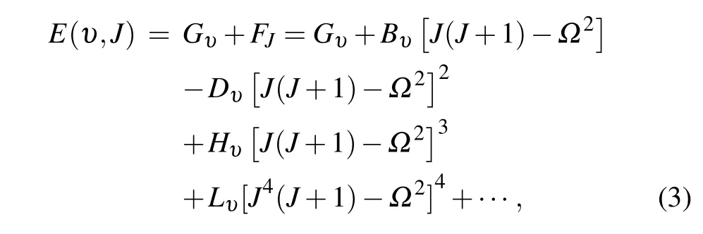
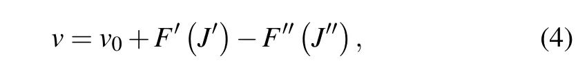
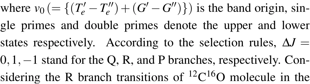
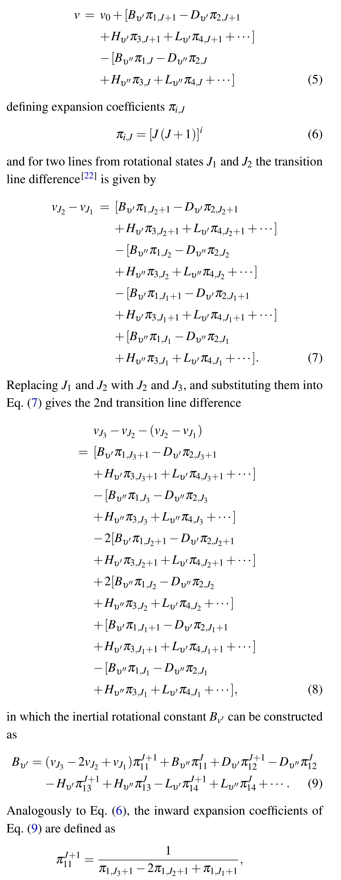
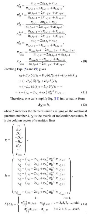
whereGυandFJcorrespond to the vibrational and rotational level, respectively.Bυ,Dυ, andHυ,...are the effective rotational and centrifugal constants.Ωis the projection of the electronic angular momentum onto the internuclear axis. The transition lines from a higher energy state to a lower energy state of a given molecule may then be written as Together equations (11) and (12) allow us to determine the{imax}(imax=even) molecular constants with{imax+3}accurate experimental transition lines. Thus, it becomes clear that the biggest challenge in calculating the argumentsχis to obtain the final form of algebraic equation (12), which offers alternative choices for the maximal degrees of the multiexpansions. Accordingly,the model described above that consists of a difference and algebraic approach (DAA) is constructed to calculate R branch transition lines.

2.2. Spectroscopy learning strategy

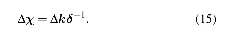
It appeared that the DAA model with fewer and explicit parameters which is desirable in the prediction of wild spectral range is better than the artificial neural networks. Therefore,understanding and characterizing the proper parametersxcan improve the overall performance of the proposed model that is generally associated with problems of avoiding under- and over-fitting. According to the DAA model, it is possible to characterize the parametersxfrom the one-to-one mapping

in which the restricted valueχwas manipulated according to the following rule:

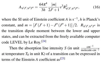
It is understood that the development of the laser spectroscopy and frequency-comb allows for precisely determined line positionsvwith high resolution, which play essential roles in determining the emission EinsteinAcoefficients for the transition from a lower state(υ′′,J′′)to an upper state(υ′,J′)[23]

wheregs,giare the state-dependent weight and state-independent weight,respectively.cis the speed of light,kis Boltzmann’s constant,Ev′′,J′′is the lower energy state,Qis the partition function atT0(=296 K), andIa(=98.6544%) is the isotopic abundance of12C16O molecule.

An alternative approach which corresponds to the calculation of line intensity of a transition at temperatureTrelies on that of reference temperatureT0[23]

Finally,it is thus devoted to explore spectroscopy learning that helps to extract the novel and hidden information from the data sets such as{vexpt},{ARef},{SRef}, where the learning and optimization algorithms can be seen in the next section.

2.3. Learning and optimization algorithms

According to Eq.(11),the DAA model embedded in spectroscopy learning algorithm is practically heuristic, yielding many possibilities for{x}, which may suffer from different optimization problems that require some effective implementation algorithms to evaluate the final determination.

Thus, to get the optimal solution, the main idea of spectroscopy learning is to find accessible and explicit rules to minimize the objective functions

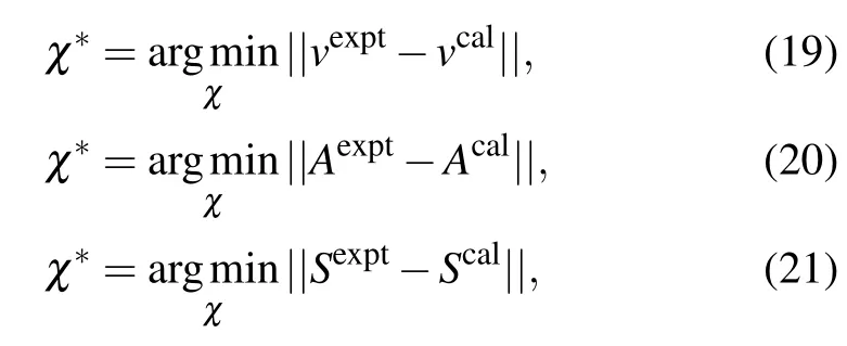
where the parametersxare unknown to be computed through Eq. (12). The Einstein coefficientAcal(χ), line intensityScal(χ) both associate strongly withxand their own definitions. In order to estimate the precision of the reconstruction,we used the residual of the root mean squares (RMS) of the deviations as the distance for transition lines

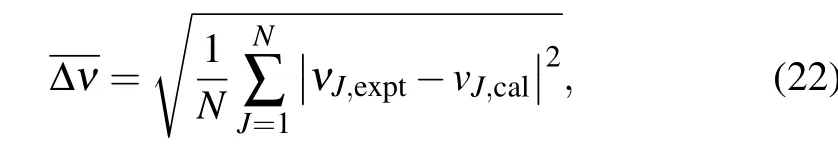
whereNis the number of data points.According to other spectroscopic quantities,the distance can be arranged into the similar forms,written as

Equations (22)–(24) listed above are straightforward optimal goals to evaluatex∗. From another point of view, there is no doubt that the EinsteinAcoefficient and line intensity are the critical basis for understanding the spectral information, and more importantly,the ideal physical convergence of extrapolative prediction. As mentioned earlier, spectroscopy that is an essential investigative technique allows for satisfactory transition lines{vexptn }with sub-MHz or even kHz accuracy,which can be used to analyze molecular constants at a local fitting by the least square strategy, however, resulting in poor ability in extrapolating line positions beyond the measurement.

In this work,the most attention of spectroscopy learning has been devoted to the optimization of parameters{x}with the experimental line positions lists to be divided into training and testing parts,where the optimization problems can be solved and designed in following two aspects.

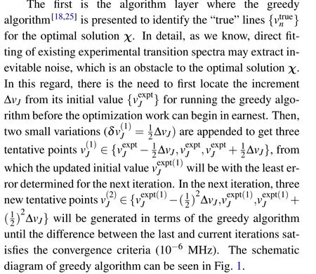
Fig. 1. The schematic diagram of greedy algorithm. The least error (right axis)for each iteration is shown.

2.4. Calculation details

Step 1 Select an initial value(e.g.,i=4),which is suggested for the correspondingχ(i).

Step 2 Record all possible alternatives, utilizing greedy algorithm in each iteration.

Step 3 Using Eqs. (22)–(24) to quantify the parametersχ(i)that best meet the corresponding threshold requirements.

Step 4 If Step 3 is done,terminate the process and currentiis the final degree of Eq.(12). Otherwise, a bigger adaptive value of degree(e.g.,i=6)will be loaded to execute and repeat Steps 1–4.

Step 5 Here,the EinsteinAcoefficient and line intensity for each line position could be generated.

3. Application

3.1. Line positions

In the present article, the spectroscopy learning method has been applied to the R-branch of 3–0 band in the ground of12C16O,where excellent examples of line positions are collected by Mondelainet al.[8]and Wanget al.[11]Moreover,the former frequencies are quoted in HITRAN2016[26]and latter ones will be updated in HITRAN2020[19]soon.Here,it is possible to test the spectroscopy learning method directly on the Wanget al.line lists(W21)[11]and the labelled line intensities and the EinsteinAcoefficients from HITRAN2020.[19]

Table 1. The determined“true”transition linesk of the 3–0 band in the ground electronic state of CO(in unit kHz).

Table 1. The determined“true”transition linesk of the 3–0 band in the ground electronic state of CO(in unit kHz).

JkvJkJkvJk 19192019842944.2622190708280671.213 21192113077706.7864190910419589.804 23192193333611.4466191099878013.489 25192260575649.4248191276620759.635 27192314768823.34210191440612666.217 0190493496458.961

Table 2. Spectroscopic constants of the 3–0 band in the ground electronic state of CO(in unit MHz).

In this work, some line lists are introduced for comparison, such as Mondelainet al. line list (M15),[8]Farrenq and Guelachvili’s line list (FG91),[3]W21 line list,[11]V12 line list,[13]CH04 line list,[14]Li’s line list(Li15).[15]Indeed, we can also make effort to reproduce the transition frequencies of P branch. Figure 2 gives the differences of the linesversus min the range−31≤m ≤30. It can be seen that an excellent agreement can be obtained between the present transition frequencies with values from measurements of M15[8]within sub-MHz accuracy and W21[11]within kHz accuracy,and with values from calculations of V12[13]and CH04[14]line lists except for FG91 set.[3]However,transition frequencies from Li’s line list[15]show poor agreement with those illustrated in Fig.2. Details of all line positions obtained which incorporate data from literature are collected in supporting information Table A1. Recently, Cyganet al.reported their results of line positions for R23,[9]R24 and R28[10]in the 3–0 band. The determined valuev(R23)=192 193 333 611 kHz is close to, but slightly higher than the Cygan’s value of 192 193 333 554 kHz.[9]We also compared the current line positions ofv(R24)=192 228 583.55 MHz andv(R28)=192 336 961.15 MHz with the results obtained by Cyganet al. withv(R24)=192 228 583.47 MHz andv(R28)=192 336 961.03 kHz,[10]verifying the accuracy of our values.

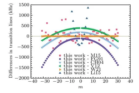
Fig.2. The differences in the transition lines for the 3–0 band. The line differences display with m=−J′′ in the P branch and m=J′′+1 in the R branch.

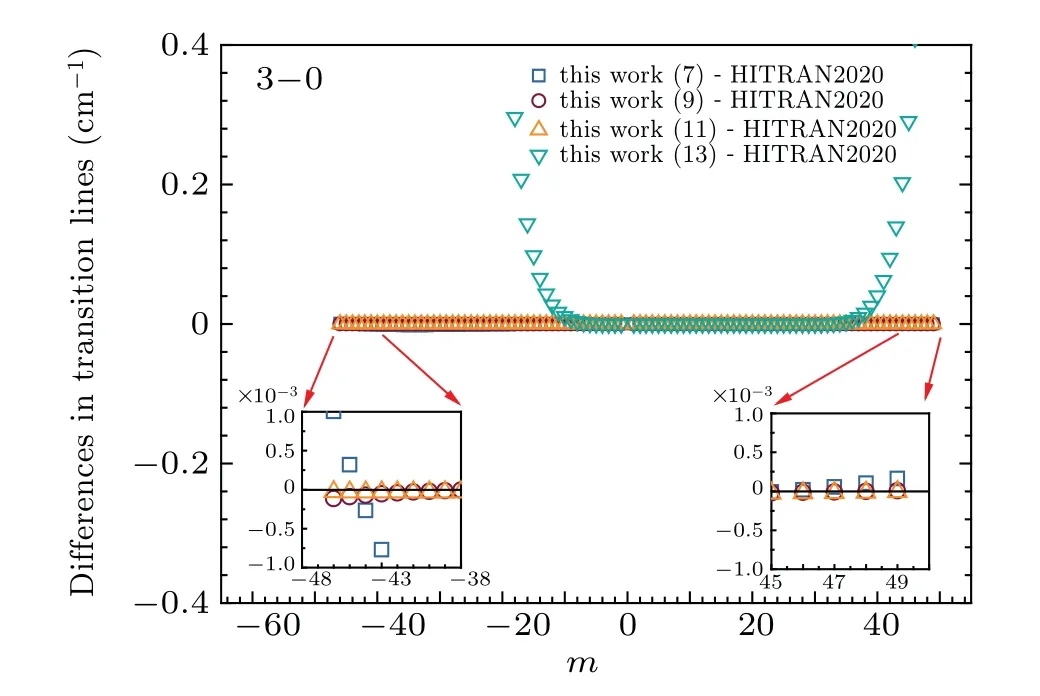
Fig.3. The differences in the transition lines of“this work(n)”and the values from the HITRAN2020 for the 3–0 band. The line differences display with m=−J′′ in the P branch and m=J′′+1 in the R branch. It should be noticed that n in“this work(n)”means n experimental lines used in the training.

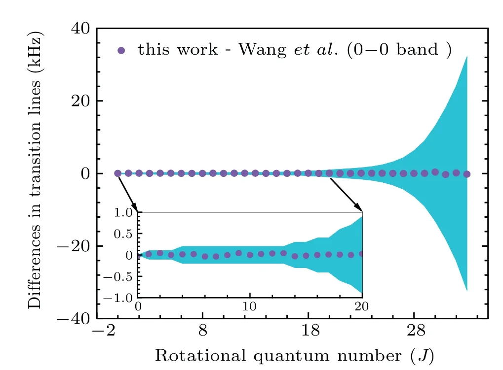
Fig. 4. The differences in the transition lines of this work and those from Wang et al.[11] for the 0–0 band. The line differences display with J′′. The color shadow covers 1–σ uncertainty region.

As already pointed out, there is diversity in DAA model which can yield line positions with different choices of spectroscopic constantsχ(i)i=4,6,8.... And, comparisons of the differences in line positions are shown in Fig. 3, where lines from “This work (11)” show a best agreement with those of HITRAN2020 line list, giving the RMS value of 2.4×10−5cm−1.

Apparently, the molecular constants with respect to the vibrational statesυ=0,−3 allow the calculations of rotational lines for 0–0 and 3–3 bands. The line differences between our results and those from Wanget al.[11]are plotted in Fig.4 and Fig.5,respectively,leading to an acceptable determination of the transition frequencies with a few kHz accuracy (see supporting information Table A2 for details).

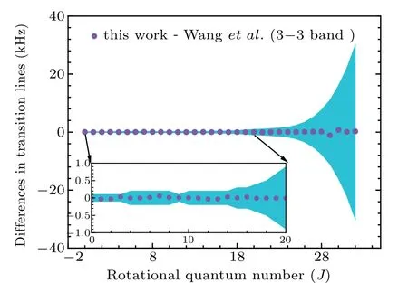
Fig.5. Differences in the transition lines of this work and those from Wang et al.[11] for the 3–3 band. The line differences display with J′′. The color shadow covers 1–σ uncertainty region.

3.2. Einstein A coefficients and line intensities

The EinsteinAcoefficients and line intensities are used to evaluate the performance of the DAA model in predicting the line positions especially those beyond the measurements. Then, according to the definitions of the EinsteinAcoefficient and line intensity(see Eqs.(16)and(17)),the potential challenge is to determine the transition dipole momentRυ′J′,υ′′J′′, which can be extracted from LEVEL[24]from the semi-empirical DMF suggested by Liet al.[15]and a PEF from Coxon&Hajigeorgiou[14]or calculated directly through Eq. (16) using EinsteinAcoefficient and transition line that both are provided by HITRAN2020 database.[19]In this work,we prefer the latter approach to confirm better predictive accuracy of the lines.

The accuracy of EinsteinAcoefficients and line intensities will be assessed by comparison between this work and those from HITRAN2020.[19]Moreover, in order to compare to literature values,several lists of EinsteinAcoefficients and line intensities are also collected, which were displayed in Fig.6 and Fig.7,respectively.And,detailed values of EinsteinAcoefficients and line intensities are presented in the supporting information Tables A3 and A4.

For the case of EinsteinAcoefficient comparisons,values from HITRAN2020,[19]G94,[12]Langhoff and Bauschlicher(LB95),[29]Hur´e and Roueff (HR96)[30]are presented. The LB95 EinsteinAcoefficient values are those calculated by Eq. (16) using the DMF suggested by Langhoff and Bauschlicher.[29]And, the HR96 EinsteinAcoefficient values are those computed by Eq.(16)using the transition dipole momentRυ′J′,υ′′J′′obtained by Hur´e and Roueff.[30]It should be noted that the lines of this work(11)were used in the calculation of EinsteinAcoefficient for both cases. The satisfactory agreement with HITRAN2020 values is viewed by the EinsteinAcoefficient comparisons plotted in Fig.6 withmbetween−46 and 49. While G94 overestimated the EinsteinAcoefficients by about average 4.4%,and the EinsteinAcoefficients of HR96 and LB95 are approximately 1.8% and 1.5%lower than calculations of this work.

Fig.6. Comparison of the Einstein A coefficients for the 3–0 band. The Einstein A coefficients display with m=−J′′ in the P branch and m=J′′+1 in the R branch.

For the case of line intensity comparison atT=296 K,values from HITRAN2020,[19]G94,[12]LB95,HR96,SV04,[7]and Borkovet al. (B20)[17]are taken in account.The G94 line intensities performed atT=296 K are computed by Eq.(18)using G94 line intensities at reference temperatureT=3000 K[12]with theQ(T=3000 K) value of 1717.24391[15]in order to foster a fair comparison with available line intensities. The LB95 and HR96 line intensities are calculated by Eq. (17) with respective EinsteinAcoefficients derived before and with theQ(T=296 K) value of 107.419824.[15]The B20 line intensities are the calculated values that can be found in supplementary material of Ref.[17].

The comparisons of line intensitiesversus mbetween−46 and 49 are shown in Fig. 7, in which the line intensity values of G94 and B20 are approximately 5.8% and 3.9%higher than present values, respectively, and the values of LB95 and HR96 are smaller than present values by about 1.5%and 1.8%,respectively. These slight discrepancies arose from that slightly different line position values and transition dipole moment are used for line intensity calculation. Whereas,line intensity values of this work are identical to the entries of the HITRAN2020 values[19]and deviate slightly from those measured by Sung and Varanasi.[7]

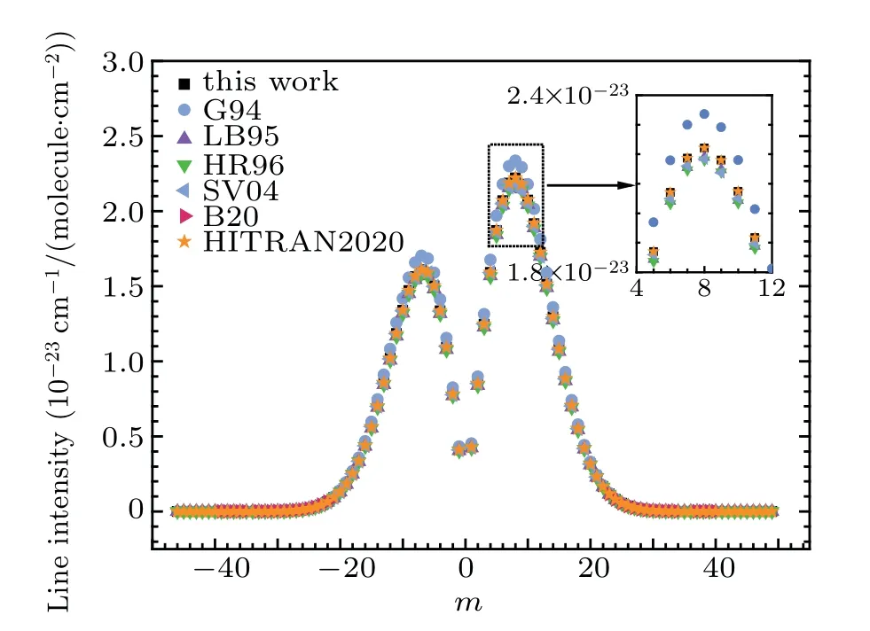
Fig.7. Comparison of the line intensities for the 3–0 band. The line intensities display with m=−J′′ in the P branch and m=J′′+1 in the R branch.

Fig.8. Comparison of the Einstein A coefficients for the 0–0 and 3–3 bands.The Einstein A coefficients display with m=J′′+1 in the R branch.

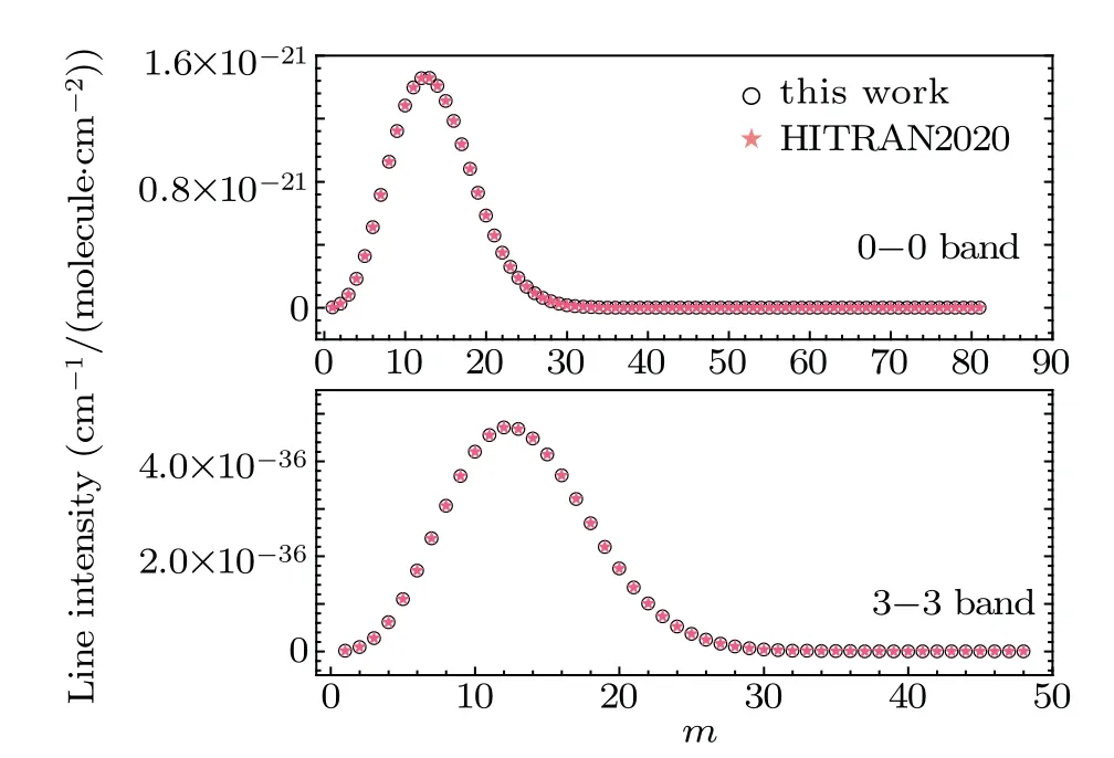
Fig.9. Comparison of the line intensities for the 0–0 and 3–3 bands.The line intensities display with m=J′′+1 in the R branch.

Let us finally consider the EinsteinAcoefficients,line intensities for the 0–0 and 3–3 bands. Now,spectroscopic constants reported in Table 2 are ready for these two tasks with the help of transition dipole momentRυ′J′,υ′′J′′that were extracted from LEVEL[24]from the semi-empirical DMF suggested by Liet al.[15]and a PEF from Coxon&Hajigeorgiou.[14]Then,solving Eqs. (16) and (17) leads to the EinsteinAcoefficients and line intensities that are consistent with those from HITRAN2020.[19]These are clearly shown in Figs. 8 and 9 that compare these two value lists for the cases of EinsteinAcoefficients and line intensities, respectively, withm=1 tom=81 for the 0–0 band,m=1 tom=48 for the 3–3 band.Those values of EinsteinAcoefficients and line intensities for the 0–0 and 3–3 bands are presented in the supporting information Tables A5 and A6.

4. Conclusions

In this article, a model- and data-driven strategy is proposed to learn line positions for diatomic molecules. The use of the strategy can help us unearth the hidden information behind the measurement and is applied for the 3–0 band in the ground electronic state of12C16O,enabling prediction with a few kHz accuracy. The present values of line positions, EinsteinAcoefficients and line intensities are compared to several other line lists, verifying the validity of the strategy. The results also suggest that the size in the learned-model can have different effects and diversities on the predictive accuracy of line positions. Moreover,in our forthcoming work,it could be interesting to see if the performance of the proposed technique is also reachable for CO isotopologues.

Acknowledgment

We appreciate Prof. V.I.Perevalov for his valuable suggestions for the line intensity calculations.