Stabilization strategy of a car-following model with multiple time delays of the drivers∗

Weilin Ren(任卫林) Rongjun Cheng(程荣军) and Hongxia Ge(葛红霞)

1Faculty of Maritime and Transportation,Ningbo University,Ningbo 315211,China

2Jiangsu Province Collaborative Innovation Center for Modern Urban Traffic Technologies,Nanjing 210096,China

3National Traffic Management Engineering and Technology Research Centre Ningbo University Subcenter,Ningbo 315211,China

Keywords: car-following model,driver’s reaction time delays,improved definite integral method,bifurcation analysis,stabilization strategy

1. Introduction

In the course of car-following behavior, time delay is an important factor affecting the stability of traffic flow. Time delay is reflected in two aspects. On the one hand, for the driver,there exists time delay from processing the information of the preceding vehicle to take corresponding measures. On the other hand, for the adaptive cruise control system, there also exists an inevitable time delay from the perception of information,and calculation to the final complete control of vehicle operation. Therefore,how time delay affects traffic flow and how to make rational use of time delay to control vehicles are issues of widespread concern in related fields.

In 1995, Bandoet al.[1]proposed the optimal velocity model (OVM). They assumed that in the process of car following, there always exists a corresponding optimal velocity according to the changes in the distance of following vehicle,and the driver’s goal is to adjust the velocity of current vehicle to approach the optimal velocity.Subsequently,Bandoet al.[2]proposed the OVM with time delay by introducing driver’s reaction delay into the OVM

whereαis the sensitivity coefficient,V(·) is the optimal velocity function, andτis the reaction delay of driver. By analyzing the stability of uniform traffic flow and simulating the dynamic behavior,a critical value of delay inducing traffic jam was obtained,and they found that traffic jam occurs when the value of delay is greater than the critical one.Since then,based on OVM,research on the impact of time delay effects on traffic flow emerged.Research can be divided into two categories.The one is delay determined, which studies the dynamic behavior of other parameters in the system.For example,Zhouet al.[3]integrated the velocity difference and optimal velocity difference of two adjacent vehicles into the OVM.Meanwhile,they assumed that a driver had the same reaction time to different stimulus,such as the velocity of the current vehicle,the velocity difference with the adjacent vehicle ahead, and the headway distance difference with the adjacent vehicle ahead.In their work, evolution trend of traffic flow stability was obtained by fixed time delay. Furthermore,Sunet al.[4]considered that the driver’s stimulus to the information of the current vehicle was different from that to the information of the preceding vehicle. Then, similar results of traffic flow stability can be obtained. In this way, studies[3,4]focused on the stability analysis of the traffic flow with fixed time delay, while ignored the important impact of time delay on traffic flow.Therefore,it is difficult to explain the inherent mechanism of congestion in time-delay traffic system.The other is to explore the nonlinear behavior of traffic flow system induced by time delay. Existing studies[5–7]have shown that bifurcation theory can well explain some sophisticated traffic dynamic behaviors caused by delay and the formation mechanism. For example,Oroszet al.[5]studied the global bifurcation behavior of a carfollowing system with time delay composed of three vehicles.The information obtained from their simulation was that the uniform traffic flow loses stability when the average headway was located in a certain region. The scale of unstable region was related to the ideal velocity and the sensitivity of driver to stimulus signal. The greater the ideal velocity of the vehicle,the weaker the sensitivity of the driver to the stimulus signal,and the larger the unstable region. Further,Oroszet al.[6]considered a time-delay system consisting of 17 vehicles. In the numerical simulation, a region where multiple periodic solutions coexist was discovered by selecting average headway as the bifurcation parameter. These different periodic solutions corresponded to different traffic flow patterns in real traffic.Furthermore, Oroszet al.[7]had increased the number of vehicles to 33 in order to explore more abundant traffic phenomena. Moreover, a bistable region induced by subcritical Hopf bifurcation was found,which consisted of uniform traffic flow pattern and traffic jam pattern.

The above mentioned theoretical studies[3–7]show that time delay may lead to complex dynamic behavior. Therefore, how to suppress the negative impact of delay effect on traffic flow system is a topic worth discussing. At present,from the perspective of control terms,various control terms are designed to suppress traffic congestion caused by time delay.For example, Liet al.[8]designed a new control term, which was composed of headway difference and velocity difference between two adjacent vehicles, to suppress the traffic oscillation caused by varying reaction-time delay of the driver. Jinet al.[9]proposed a delayed feedback control term consisting of the difference between the current velocity and headway and the historical ones. Zhouet al.[10]added velocity difference of historical moment between two adjacent vehicles as control term into the system. However, there is a defect in these works.[8–10]That is,the specific design of control parameters is not fully reflected. To address this gap,Jinet al.[11]applied the definite integral stability method to determine the stable interval of the single control parameter. To sum up, most of the studies have the following gaps: (i)emphasis is placed on the design of control terms, while ignored the design of control parameters;(ii)in the process of modeling driver’s driving behavior,the delay concerning driver’s reaction is not considered,which have a dramatic impact on the control effect;(iii)the design of control parameters is difficult to apply in actual scenarios due to redundant iterations. Therefore, this paper will comprehensively design the control term and parameters in the term, in order to mitigate the unstable traffic flow induced by driver’s reaction time delay.

The specific contribution of this paper are as follows:

(I) In the design of control strategy, the influence of driver’s reaction time delay to different stimulus is considered,which is closer to the actual traffic situation.

(II) Based on the bifurcation theory, the definite integral stability method is improved, for which the redundant iterations in the original method are eliminated and the application value is enhanced. Meanwhile,the improved definite integral stability method is successfully applied to one-dimensional and three-dimensional parameter spaces.

The remainder of this paper is organized as follows. In Section 2, an extended full velocity difference model considering driver’s reaction time delays is proposed to describe the driver’s driving behavior,and its stability is analyzed. In Sections 3 and 4,the control term and the parameters in the term are designed respectively. In Section 5, the measured data is leveraged to verify the effectiveness of control strategy. In Section 6,our conclusions are discussed.

2. Mathematical model and stability analysis

2.1. Mathematical model

At present, the modeling of time delay based on carfollowing models is sufficient.[4,12]In 2018, the general nonlinear car-following model with multi-time delays was proposed by Sunet al.[4]Mathematical model was expressed as follows:

where ∆xn(t −τ1) =xn+1(t −τ1)−xn(t −τ1) denotes the headway distance between then-th vehicle and the preceding vehiclen+1 att −τ1,vn(t −τ2) is the velocity of then-th vehicle att −τ2, ∆vn(t −τ3)=vn+1(t −τ3)−vn(t −τ3) denotes the velocity difference betweenn-th vehicle andn+1-th vehicle att −τ3, andτ1,τ2, andτ3represent the driver’s reaction time delay to headway distance, velocity and velocity difference,respectively.

Equation (2) specifies varieties of car-following models.[13,14]In this paper, full velocity difference model(for short, FVDM) is selected to describe the car-following behavior of human-driven vehicle. Therefore, equation (2) is rewritten as

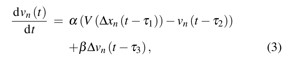
whereαandβrepresent the sensitivity coefficient of the driver to the velocity difference, andV(·) is the optimal velocity function. In this paper,the following form of optimal velocity function proposed by Bando[1]is adopted as

wherehcdenotes safe headway,θ1andθ2are the dimensionless coefficients used to determine the shape of the optimal velocity. In the simulation of Sections 3 and 4,the parameters inV(∆xn(t)) are[1]vmax=33.6 m/s,θ1=0.086,hc=25 m andθ2=0.913.

Note that the full velocity difference model with multiple time delays(i.e.,Eq.(3))is called as FVDM-MTD for short.

2.2. Linear stability analysis

In this section, linear stability analysis is performed to derive the stability condition of FVDM-MTD without control scheme. Assume thatNvehicles are placed on a ring-road of lengthL. Thereby,the constant headway can be expressed ash∗=L/N. For uniform traffic flow, all vehicles maintain the identical headway distance and velocity,which can be expressed as

Ifz2>0 holds,the uniform traffic flow is stable for small disturbances. Thereby, the stability condition for FVDMMTD can be expressed as

Equation (11) is an important prerequisite for the subsequent design of feedback control. If the stability condition(i.e., Eq. (11)) is not satisfied during vehicle operation, the feedback control designed will work.

3. The design of feedback control term and bi-

furcation analysis

3.1. Control scheme

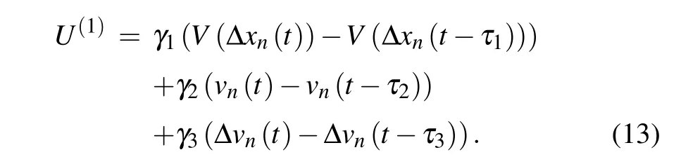
In this section,the design of feedback control term is performed. The core of the design is to form the control signals by the difference between the current state and the historical state of the system. Thereby,the general form of control term can be expressed as

whereγ1,γ2, andγ3denote feedback gain of velocity difference, optimal velocity difference and difference of velocity difference,respectively,whileτc1,τc2,andτc3denote the design time delay corresponding toγ1,γ2, andγ3, respectively.Obviously, there are six parameters (i.e., feedback gains and time delays)to be determined in Eq.(12). In order to clearly embody the principle of the design, the control terms corresponding to Eq.(12)are evolved into two cases.

Case 1 In this case,it is assumed that the driver’s reaction time delay can be estimated or detected by on-board equipment. Therefore, the design time delayτc1=τ1,τc2=τ2,andτc3=τ3are known, and the feedback gains (i.e.,γ1,γ2,andγ3)are need to be determined,which will be elaborated in Section 4. Thereby,Eq.(12)is rewritten as

Case 2 Assume that the feedback gains are set in advance.Unify the design time delay to be determinedτc1=τc2=τc3=τm. Therefore,Eq.(12)can be expressed as

3.2. Bifurcation analysis

In this section,bifurcation analysis on controlled FVDMMTD is performed to investigate the distribution of eigenvalues when Hopf bifurcation occurs.

The following controlled FVDM-MTD is selected to demonstrate the procedure of bifurcation analysis:

wheref(·)=α(V(∆xn(t −τ1))−vn(t −τ2))+β∆vn(t −τ3)denotes driver’s driving behavior,andU(1)(i.e.,Eq.(13))represents driver assistance controller,which helps the driver adjust the operation state of the vehicle. For simplicity, we setτ3=τ1.[4]The state errors of then-th vehicle around the equilibrium states can be expressed as

By inserting Eq. (16) into Eq. (15), a vectorized matrix with regard to FVDM-MTD can be obtained

whereδy(t)=[δv(t),δx(t)],δx(t)=[δx1(t),...,δxN(t)],andNis the total number of vehicles on the ring-road. The block matrices in Eq.(17)are expressed as

Insertingλ=µ+iω(where i is the imaginary unit,µis the real part andωis the imaginary part)into Eq.(21)and separating the real and imaginary parts yield

wherec1= cos(τ1ω),c2= cos(τ2ω),ck= cos2kπN,s1=sin(τ1ω),s2=sin(τ2ω),andsk=sin(2kπ/N),

Note thatk ∈{1,2,...N}denotes the wave number. Fork=N, (µ,ω)=(0,0) is one of the roots and another root depends on the parameters. That is, for arbitrary parameters andk=N, there always exists the eigenvalueλ=0 in the system, which leads to the translational symmetry,[15,16]as shown in Fig. 1. Therefore, the real parts of characteristic root forkandN −kare equal, whereas the imaginary parts are opposite. Due to the existence of translational symmetry,we only focus on the movement of curves corresponding tok ≤(N −1)/2 (i.e.,k=1,2,3 in Fig. 1). Figures 1(a) and 1(b) show the distribution of characteristic roots of uncontrolled and controlled FVDM-MTD, respectively. In Fig. 1,the curve corresponding to eachk ∈{1,2,...,N −1}consists of left branch and right one. AsV′increases,the curves move in the direction indicated by the arrow. From Fig. 1(a), the right branch corresponding tok=1 first crosses the imaginary axis, and those corresponding tok=2 andk=3 fail to cross the imaginary axis but have a tendency to cross the imaginary axis. Whereas, for the controlled FVDM-MTD with fixed(γ1,γ2,γ3)=(0.1,0.3,0.2), the curves corresponding tok ∈{1,2,3}stay in the left plane. Meanwhile,the real part of the eigenvalue of the system is related to the stability of the system. That is,if the real part is greater than zero,the system is unstable, otherwise the system is stable. Therefore, compared with Figs. 1(a) and 1(b), it is clear that the controlled system can delay or hinder the generation of unstable eigenvalues.

Fig. 1. The distribution of real and imaginary part of eigenvalues for uncontrolled FVDM-MTD and controlled FVDM-MTD with fixed N = 7,α =1 s−1,β =0.5 s−1,τ1=0.5 s and τ2=0.3 s.

Fig.2. The distribution of real and imaginary parts of eigenvalues of the system(15)with k=1,N=7,α =1 s−1,β =0.5 s−1,τ1=0.5 s,τ2=0.3 s.

In particular,Oroszet al.[15]found thatk=1 corresponds to stability condition of uniform traffic flow, while fork>1,further oscillation modes appear around the already unstable equilibrium. The conclusion drawn by Orosz is consistent with what is shown in Fig. 1. That is, the curve represented byk=1 breaks through the imaginary axis faster than other curves withk>1, which means the stability of the system can be judged by the case ofk=1. Therefore,combing with Eq. (22), the study on distribution of eigenvalues of the system(15)can be simplified as the casek=1,as shown in Fig.2.In Fig. 2, the blue line represents the uncontrolled FVDMMTD (i.e., (γ1,γ2,γ3) = (0,0,0)), while the red and green lines represent the controlled FVDM-MTD,corresponding to(γ1,γ2,γ3)=(0.1,0.3,0.2)and(γ1,γ2,γ3)=(0.8,0.4,0.5),respectively. Obviously, the right half of the blue line crosses the imaginary axis first with the increase ofV′, where the intersection of the blue line and the imaginary axis is the bifurcation point. That is,compared with controlled FVDM-MTD,the uncontrolled one is more prone to be affected by disturbances,resulting in unstable traffic flow. The right half of the green line is very close to the blue one,and similar to the blue line,the left half of the green line crosses the imaginary axis.In contrast, the right half of the red line retains more parts in the second quadrant than the green line and the blue line.More importantly, the entire left half of the red line remains in the third quadrant, without crossing the imaginary axis. That is,the control effect of the parameter combination represented by the red line exceeds that of the green line. Furthermore, the appropriate combination of control parameters can suppress the unstable traffic flow caused by driver’s time delay. Therefore, how to choose the appropriate combination of control parameters is an interesting problem, which will be solved in Section 4.

4. The design of parameters in feedback control term

In this Section,we will explore how to choose the appropriate combination of parameters to postpone or eliminate the negative impact of driver’s time delay on the traffic flow.From Section 3,it is noted that the real part of the eigenvalue has a dramatic influence on the stability of the system. Therefore,the eigenvalue of the system is a breakthrough worthy of attention. However,the characteristic equation of the system is a transcendental equation (such as Eq. (21)), which is difficult to solve directly. To overcome this gap,a definite integral stability (for short, DIS) method is proposed by Jinet al.[11]However, in practical applications, there are redundant iterations in the DIS method,which will prolong the computation time. That is, the DIS method determines the stability of the system by calculating the number of positive real parts of the eigenvalues for all possiblek. Inspired by Fig.1 and Ref.[15],we propose an improved definite integral stability (for short,IDIS)method by focusing on the property of system fork=1 and ignoring that fork>1. It can be known from Fig.1 and Ref.[15]that the curve withk=1 crosses the imaginary axis faster thank>1. That is, the stability of the system can be determined byk=1 instead of solving the eigenvalues for all possiblek. The procedures of the IDIS method are as follows.

Step 2 Determine integral functionC(ω) by the following formula:

Set the value of common parameters asα= 0.6 s−1,β=0.5 s−1,τ1= 0.5 s,τ2= 0.4 s,N= 7,h∗= 25 m, andV′(h∗)=1.448.

According to Eq. (11), 1.448×(0.4−0.5−(1/0.6))+((0.5/0.6)+(1/2)) =−1.2248< 0 dissatisfies the stability condition. Subsequently, we will utilize the abovementioned steps to design the feedback gain and design time delay in the control term,in order to alleviate the oscillation caused by unstable traffic flow.

4.1. The design of feedback gain and its verification

We first adopt the control term (i.e., Eq. (13)) described in case 1,where the design time delays are known(i.e.,τc1=τc3=τ1=0.5 s andτc2=τ2=0.4 s). Therefore, the controlled FVDM-MTD can be expressed as follows:

Fig. 3. The stability diagram of different feedback gain combinations(γ1,γ2,γ3) for controlled FVDM-MTD with fixed design time delay and N=7.

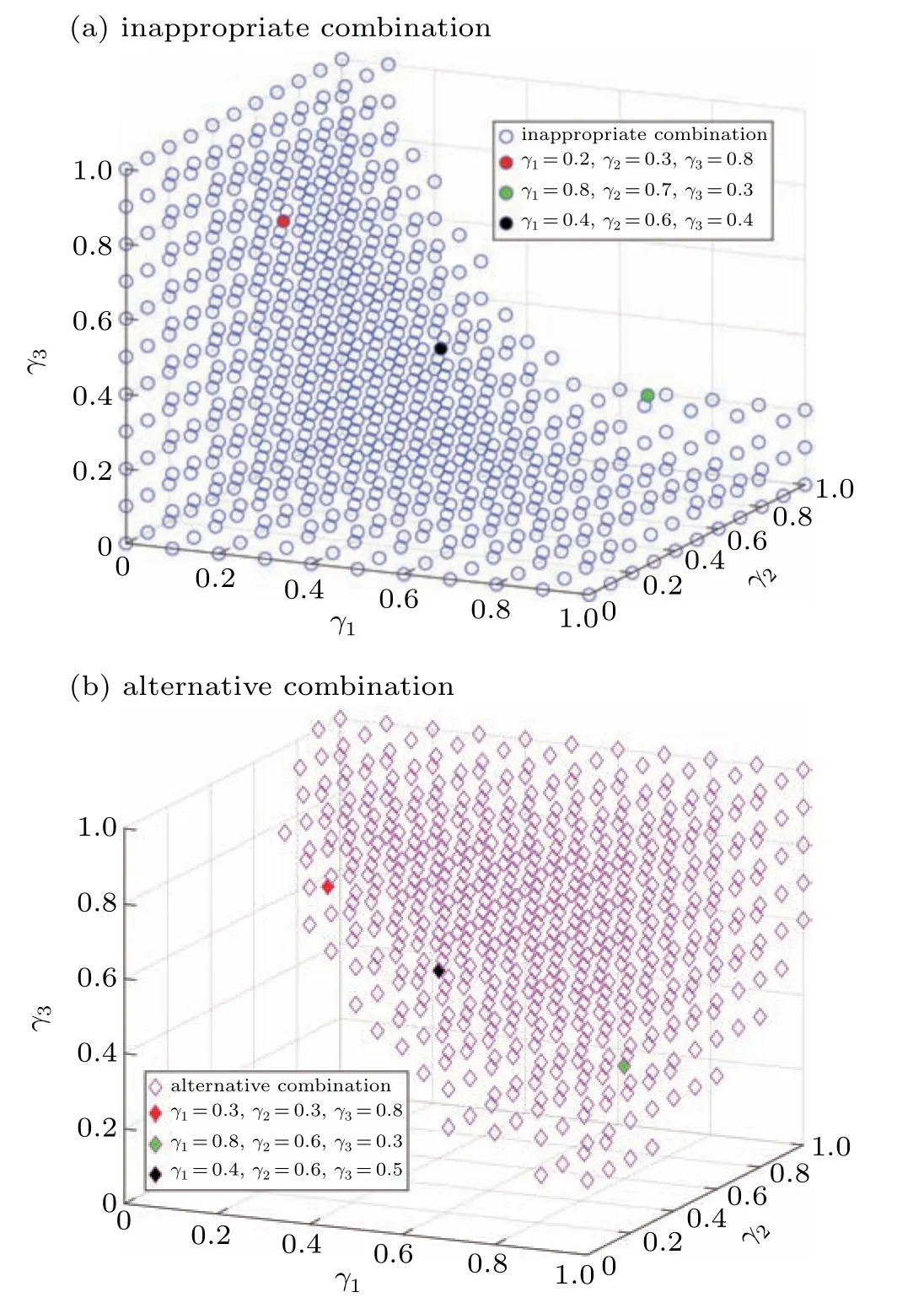
Fig.4. The corresponding decomposition diagram of Fig.3: (a)shows all inappropriate combinations in Fig.3; (b)portrays all alternative combinations in Fig.3.

Fig. 5. Velocity evolution of the first car for different feedback gain combinations in Fig. 4: (a) involves the parameter combinations represented by the red dot;(b)involves the parameter combinations represented by the green dot;(c)involves the parameter combinations represented by the black dot.

According to Eq.(29)and detailed steps 1–4,the stability diagram for the controlled FVDM-MTD is plotted in(γ1,γ2,γ3)∈[0,1]×[0,1]×[0,1],as shown in Fig.3. In Fig.3,the blue circle represents an inappropriate combination of feedback gain(i.e.,Ω(γ1,γ2,γ3)=1),whereas the pink diamond represents an alternative combination (i.e.,Ω(γ1,γ2,γ3)=0) to eliminate the oscillation induced by unstable traffic flow. In order to illustrate the effect of control strategy more clearly,the corresponding decomposition diagram of Fig. 3 is drawn, as shown in Fig. 4. Figure 4(a) depicts the distribution of inappropriate combinations,and Fig.4(b)portrays the distribution of alternative combinations. Then, we validate the effect of control strategy by selecting three points from Figs. 4(a) and 4(b),respectively. It can be seen from Fig.5 that the combination of feedback gains from Fig. 4(b), such as (γ1,γ2,γ3)=(0.3,0.3,0.8), (γ1,γ2,γ3) = (0.8,0.6,0.3) and (γ1,γ2,γ3) =(0.4,0.6,0.5)can well reduce the variation of the velocity fluctuations. Conversely,when adopting the combination of feedback gains in Fig.4(a),the velocity fluctuation of the first vehicle increases gradually and eventually forms a dense equalamplitude oscillation with the small disturbance added.

From Figs. 3–5, the feasibility and effectiveness of the design of feedback gains of controlled FVDM-MTD has been verified.

4.2. The design of design time delay and its verification

In this section,the control term in case 2(i.e.,Eq.(14))is leveraged to restrain unstable traffic flow. The corresponding controlled FVDM-MTD is given as

Similar to the design of feedback gains mentioned in Subsection 4.1, according to Eq. (31), the stability interval of the controlled FVDM-MTD with respect to the design time delay can be obtained,as shown in Fig.6. The stability interval is roughly located atτm∈[0.47,0.98]. Within the stable interval, the design time delaysτm=0.6 s, 0.7 s, and 0.8 s are selected to simulate and analyze the effectiveness of the control strategy. As shown in Fig. 7, the control strategy within the stability interval can well mitigate the initial perturbation until the velocity fluctuation tends to a horizontal line. Then,we take a point on the left and right sides of the left critical point of the stability interval,such asτm=0.45 s(from unstable interval)andτm=0.47 s(from stable interval). Similarly,τm=0.98 s (from stable interval) andτm=1 s (from unstable interval)can be obtained on the left and right sides of the right critical point. As can be seen from Fig. 8, the trends of velocity fluctuation at both sides of the critical point are significantly different. When the values of design time delay are in the stable interval, the amplitude of speed fluctuation decreases gradually, while when the values cross the critical point to reach the unstable interval, the amplitude increases gradually, which fully demonstrates the effectiveness of the control strategy for design time delay.

Fig. 6. The stability diagram of different design time delays for controlled FVDM-MTD with fixed feedback gain and N=7.

Fig. 7. Velocity evolution of the first car for different design time delays instability interval in Fig.6.

Fig.8. Velocity evolution of the first car for different design time delays near the critical point of stable interval in Fig.6.

5. Case study

5.1. Parameter calibration of uncontrolled FVDM-MTD

In order to verify the practicability of the control strategy mentioned in Sections 3 and 4, partial measured data of Next Generation Simulation (for short, NGSIM) is leveraged in this section to calibrate the parameters of the FVDM-MTD reflecting the driver’s driving behavior.

NGSIM[17]is a project conducted by the Federal Highway Administration in 2002, in order to provide data support for the establishment and the validation of microscopic traffic models. NGSIM collects data through video,in which the image information of traffic flow on a highway is recorded at a frequency of 10 frames per second,and the image information is extracted into data information,including the vehicle’s location,speed,etc. According to the data filtering rules proposed by Chenet al.,[18]a dataset containing 1080 sets of data is extracted for subsequent parameter calibration.

Firstly,grey relational analysis(GRA)[19,20]is leveraged to determine driver’s reaction delay,which includes the delayτ1for the headway (∆xn(t)), the delayτ2for the velocity of following vehicle(vn(t))as well as the delayτ3for the velocity difference between adjacent two vehicles (∆vn(t)). GRA is based on the development trend of two factors. Therefore,the relationship between the acceleration of the follower vehicle(an(t))and ∆xn(t −τ1),vn(t −τ2)as well as ∆vn(t −τ3),in whichτ1,τ2,τ3∈[0.1,3],is investigated according to GRA and dataset. The relational grades of factors are shown in Fig. 9, where the higher the relational grade, the higher the correlation with accelerationan(t). From Fig. 9, ∆xn(t −1),vn(t −0.3)and ∆vn(t −0.4)have the highest correlation withan(t), thereby the driver’s reaction delays are determined asτ1=1 s,τ2=0.3 s,andτ3=0.4 s.

Fig.9. Schematic diagram of relational degree between various factors and acceleration.

Next,based on the structure of the model and the known input and output variables, genetic algorithm (GA)[21]is applied to determine the remaining pending parameters of FVDM-MTD. The dataset above mentioned is averagely divided into dataset 1 and dataset 2,each containing 540 sets of data. The model to be calibrated is represented as follows:

See Table 1 for the configuration of GA.See Table 2 for range of parameters.

The parameters of Eqs. (32) and (33) are calibrated by combining GA with dataset 1. The calibration results are shown in Table 3 and Fig. 10. Subsequently, we validate the calibration results by using dataset 2, and the value of EC is 0.7344,which is an accepted value,indicating that the calibration results can be used for subsequent verification of control strategy.

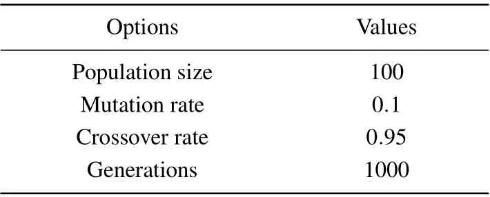
Table 1. The configuration of GA.

Table 2. The range of parameters.

Table 3. The calibration results of parameters.

Fig.10. Contrast of acceleration between fitting data and measured data.

5.2. Application and verification of control strategy

According to the results of parameter calibration and the stability condition (i.e., Eq. (11)), 1.1593×(0.3−1−(1/0.4168)) + ((0.9131/0.4168)+(1/2)) =−0.9022< 0 holds, which indicates that the traffic flow is in an unstable state. Next, we will verify whether the control strategies designed in Sections 3 and 4 can effectively suppress the unstable traffic flow. Firstly, a simulation scene is constructed as 100 vehicles run on a ring-road of length 2080.17 m.

(1) Control term of case 1 as well as the design of feedback gains.

The formula of controlled FVDM-MTD is as follows:

Combined with DIIS algorithm and Eq. (36), the stability of the controlled FVDM-MTD with different combinations of feedback gains is illustrated in Fig. 11. Figure 12 is a decomposition of Fig. 11, where Fig. 12(a) consists of all inappropriate combinations and Fig. 12(b) is composed of all appropriate combinations. Select two inappropriate combinations from Fig.12(a), such as(γ1,γ2,γ3)=(0.1,0.4,0.6)and(γ1,γ2,γ3)=(0.5,0.7,0.2), and one appropriate combination from Fig.12(b),such as(γ1,γ2,γ3)=(0.6,0.3,0.8). What reveals in Fig. 13 is velocity evolution of all vehicles for three selected combinations applied to control unstable traffic flow.It can be seen from Fig.13 that the combinations represented by red and green lines fluctuates violently at 2000 s,while the combination represented by blue line shows a horizontal state,which indicates the effectiveness of the control strategy.

Fig. 11. The stability diagram of different feedback gain combinations(γ1,γ2,γ3) for controlled FVDM-MTD with fixed design time delay and N=100.

Fig.12. The corresponding decomposition diagram of Fig.11.

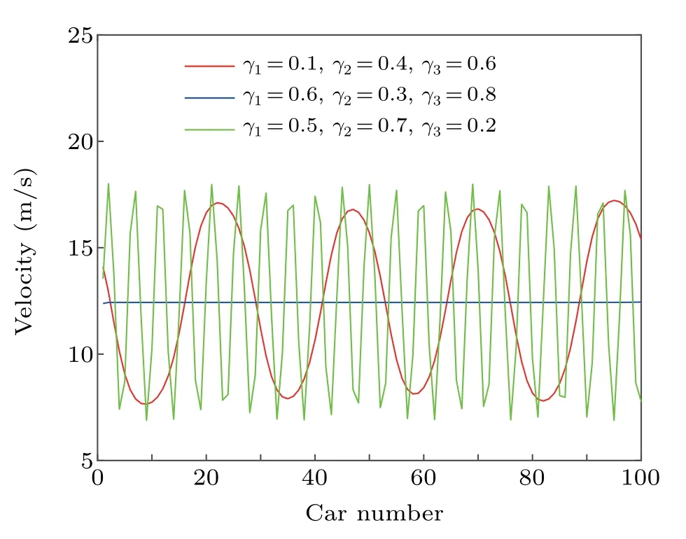
Fig. 13. Velocity evolution of all vehicles at 2000 s for different feedback gain combinations in Fig.12.

Fig. 14. The hysteresis loops of the controlled FVDM-MTD correspond to Fig.13.

Figure 14 shows the hysteresis loops of the control FVDM-MTD with different combinations. The weaker the influence of disturbance on steady-state traffic flow, the smaller the hysteresis loop effect. Clearly, when the appropriate combination (i.e., (γ1,γ2,γ3)=(0.6,0.3,0.8)) is used,as shown in Fig. 14(a), the hysteresis loop degenerates to a point,which is identical with the trend of velocity fluctuation shown in Fig.13.

Figure 15 shows a comparison of the velocity evolution of all vehicles between controlled FVDM-MTD (i.e.,γ1=0.6 s−1,γ2=0.3 s−1,γ3=0.8 s−1)and uncontrolled FVDMMTD(i.e.,γ1=0 s−1,γ2=0 s−1,γ3=0 s−1)from 1900 s to 2000 s. Obviously,multiple local cluster waves are formed in Fig. 15(b), whereas in Fig. 15(a) frequent stop-and-go waves disappear due to the addition of a control term with appropriate feedback gain combination, which demonstrates that a reasonable design of feedback gains can indeed mitigate the negative impact of driver’s time delay.

Fig. 15. Comparison between the controlled FVDM-MTD and the uncontrolled.

(2)Control term of case 2 as well as the design of design time delay.

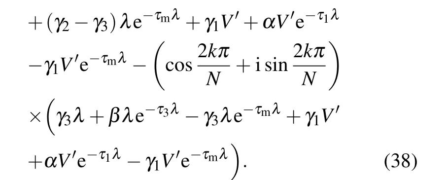
The corresponding characteristic equation of Eq.(37)is as follows:

Similarly, for fixed feedback gains, an alternative range of design time delay is depicted, as shown in Fig. 16. Takeτm=0.5 s from the stable interval(i.e.,Ω=0)of Fig.16 andτm=0.2 s from the unstable interval(i.e.,Ω=1)of Fig.16.By simulating the velocity evolution of all vehicles for the controlled FVDM-MTD with different design time delay att=2000 s, it is found that the inappropriate design time delay represented by the red line in Fig.17 still fluctuates,while the appropriate one represented by the blue line maintains a horizontal line,which indicates that all vehicles in the system are in equilibrium state,and the initial disturbance eventually dissipates. Hysteresis loops simulated in Fig. 18 also further verify the effectiveness of the design. In Fig. 19, by comparing the uncontrolled FVDM-MTD(i.e.,τm=0 s)with the controlled one(i.e.,τm=0.5 s),it is clear that the controlled one successfully suppresses the stop-and-go wave generated by the original uncontrolled one.

Fig.16. The stability diagram of different design time delays for controlled FVDM-MTD with fixed feedback gain and N=100.

Fig. 17. Velocity evolution of all vehicles at 2000 s for different feedback gains combinations in Fig.16.

Fig. 18. The hysteresis loops of the controlled FVDM-MTD correspond to Fig.17.

Fig. 19. Comparison between the controlled FVDM-MTD and the uncontrolled FVDM-MTD.

6. Conclusion

In this paper, we firstly construct an extended carfollowing model related to driver’s reaction time delay and obtain the corresponding stability condition. In order to assist the driver steer vehicle, a new control strategy including the designs of control terms and the parameters in the terms is proposed. According to the error between the current information and the historical information of the vehicle,the design of control terms is performed. Through the bifurcation analysis of the controlled system,it is obvious that the influence of different combinations of parameters on the system is significantly different. Therefore,according to the improved definite integral stability method,the reasonable value of the undetermined parameters in the control terms is determined to improve the stability of traffic flow. The results of verification on control strategy show that the control strategy can effectively avoid traffic congestion and eliminate the negative impact of driver’s delays. This also indicates that the control strategy can be applied into the actual traffic scene, and has reference value for the design of controller of intelligent vehicle.