Abundant different types of exact soliton solution to the (4+1)-dimensional Fokas and(2+1)-dimensional breaking soliton equations

Sachin Kumar, Monika Niwas, M S Osmanand M A Abdou

1 Department of Mathematics,Faculty of Mathematical Sciences,University of Delhi,Delhi-110007,India

2 Department of Mathematics, Faculty of Science, Cairo University, Giza 12613, Egypt

3 Department of Mathematics,Faculty of Applied Science,Umm Alqura University,Makkah 21955,Saudi Arabia

4 Department of Physics, College of Sciences, University of Bisha, P.O.Box 344, Bisha 61922, Saudi Arabia

5 Department of Physics, Faculty of Science, Mansoura University, 35516 Mansoura, Egypt

6 Authors to whom any correspondence should be addressed.

Abstract The prime objective of this paper is to explore the new exact soliton solutions to the higherdimensional nonlinear Fokas equation and (2+1)-dimensional breaking soliton equations via a generalized exponential rational function (GERF) method.Many different kinds of exact soliton solution are obtained,all of which are completely novel and have never been reported in the literature before.The dynamical behaviors of some obtained exact soliton solutions are also demonstrated by a choice of appropriate values of the free constants that aid in understanding the nonlinear complex phenomena of such equations.These exact soliton solutions are observed in the shapes of different dynamical structures of localized solitary wave solutions, singular-form solitons, single solitons,double solitons,triple solitons,bell-shaped solitons,combo singular solitons,breather-type solitons,elastic interactions between triple solitons and kink waves, and elastic interactions between diverse solitons and kink waves.Because of the reduction in symbolic computation work and the additional constructed closed-form solutions,it is observed that the suggested technique is effective,robust,and straightforward.Moreover, several other types of higher-dimensional nonlinear evolution equation can be solved using the powerful GERF technique.

Keywords: nonlinear evolution equations, soliton solutions, exact solutions, generalized exponential rational function method, solitary waves

1.Introduction

Nonlinear evolution equations (NLEEs) have been extensively utilized to describe complex nonlinear physical phenomena in various fields of mathematical physics such as plasma physics, oceanography, ion acoustics, atmospheric waves, condensed-matter physics, fluid dynamics, mathematical materials science, mathematical biology, and so on.Several researchers and mathematicians have paid much attention to obtaining exact rational solutions and closed-form solutions of numerous nonlinear models of NLEE.In the process of doing so,various powerful and efficient analytical mathematical methods have been developed for finding exact analytical solutions, for example, the Bäcklund transformation method[1],the Darboux transformations method[2],the inverse-scattering method [3],the Hirota bilinear method [4],the auxiliary equation method [5], the exp-function method[6], the Lie symmetry method [7–11], the modified F-expansion method [12], modified simple equation methods[13], the-expansion method [14, 15], the generalized exponential rational function method [16, 17], and so on.Closed-form solutions of NLEEs play a significant role in our understanding of the dynamical structures and characteristic properties of various nonlinear models.Closed-form solutions to NLEEs play a key role in nonlinear physical science,as they can give us more physical information and understanding of the physical aspects of a problem.The nonlinear wave phenomena of dissipation, dispersion, reaction, diffusion, and convection are essential parts of the corresponding nonlinear wave equations.It is well known that nonlinear wave–wave interactions redistribute wave energy over the spectrum, on account of an exchange of energy resulting from resonant sets of wave components.Two processes are important due to their inclusion of nonlinear wave–wave interactions in wave models:four-wave interactions in deep and intermediate waters(known as quadruplets) and three-wave interactions in shallow water(triads), both of which have been described by Neill and Hashemi [18].In the fields of nonlinear sciences and soliton theory, see, for example, [19–22], which include further relevant nonlinear wave–wave interaction, breather wave, and super regular breather wave papers.

Solitary wave solutions and multiple solitons of different types obtained from the generated solutions are exhibited by assigning appropriate values to the unknown free constants and variables.Solitons/solitary waves are particular types of traveling wave that are not destroyed when they strike other similar types of solitary wave[23–31].Many different types of exact rational solution for the forms of solitons have attained much attention from researchers/mathematicians interested in the dynamics of solitons, the dynamical structures of multiple solitons,interaction solutions,the properties of solitons,and so on.In this paper,we aim to obtain the exact soliton solutions of the(4+1)-dimensional Fokas equation and(2+1)-dimensional breaking soliton equation via the generalized exponential rational function method.First, we consider a (4+1)-D Fokas equation [32–34] given by

where u is a wave amplitude function of the variables x,y,z,w and the temporal variable t.Fokas first introduced the higherdimensional nonlinear wave equation(1)through extended Lax pairs of integrable Kadomtsev-Petviashvili (KP) and Davey-Stewartson (DS) equations [35].The Fokas equation can be used to model internal waves and surfaces in rivers with disparate physical conditions and elastic and inelastic interactions.In nonlinear solitary wave theory,KP and DS equations can be used to describe surface waves and internal waves in straits or channels of varying depth and width, respectively.The importance of the Fokas equation arises from the physical applications of the KP and DS equations.Thus, the Fokas equation can be adapted to depict a number of phenomena in ocean engineering, fluid mechanics, optical fiber communications,and many others.In particular,this Fokas equation(1)is used to represent internal and surface waves in canals.

Another nonlinear evolution equation considered in this work is the(2+1)-D breaking soliton(BS)equation,given as follows:

which was introduced by Calogero and Degasperis [36, 37]and is used to describe the interaction of a Riemann wave propagating along the y-axis with a long wave along the x-axis.This equation (2) can be used to describe the interaction of disseminating Riemann waves.The (2+1)-D BS equation has been investigated using the Hirota direct method and a variety of other methods[38–42].Geng et al[43]recently obtained the Abel-Jacobi coordinates and the scattering coordinates.

Localized solitary waves,multiple solitons,breather types,lump types, rough waves, and the interaction solutions of the (4+1)-D Fokas equation have been studied in [44–50].In addition,the dynamical structures of solitons,lump types,rough waves,solitary waves,kink waves,and interaction solutions of the (2+1)-D BS equation have been investigated in [51–53].

In this study,the generalized exponential rational technique is utilized on two different types of NLEE,namely,the(4+1)-D Fokas equation and the (2+1)-D BS equation, and many different types of exponential rational function solution are obtained.The solutions constructed are general in formulation,and all the solutions are entirely new and have never been reported previously in existing related papers.The dynamical structures of some of the new solitary wave solutions are demonstrated graphically as well as analytically,which is helpful for researchers/mathematicians aiming to understand the complex physical phenomena of such nonlinear models.

The framework of this paper is as follows:the key stages of the proposed analytical GERF method are discussed in section 2.We obtain various families of exact soliton solution for equations (1) and (2), and the dynamical structures of the obtained soliton solutions are demonstrated in the shape of multiple solitons, breather types, and elastic interactions between solitons with kink waves via 3D graphics using the mathematical software Wolfram Mathematica in section 3.In section 4, the physical interpretations of the obtained results are addressed.Finally, conclusions regarding the results obtained are given in section 5.

2.An overview of the GERF method

We illustrate the key steps of the GERF method as follows:

· Let us consider the standard nonlinear partial differential equations (PDE), as follows:

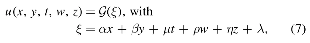
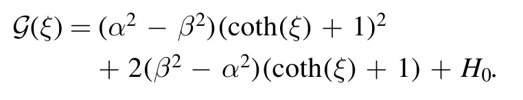
Employing the traveling wave transformationu(x,y,t,w,z) = G(ξ) ,where ξ=α x+β y+μt+ρ w+η z+λ,the standard NPDEs are then converted into the following ordinary differential equation (ODE)

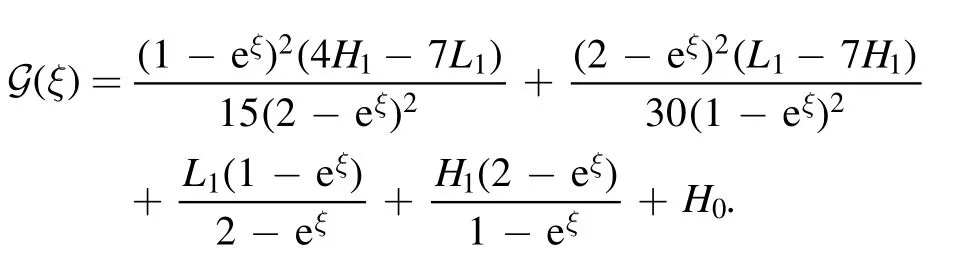
· Let us assume that the solution of (4) can be written as follows:

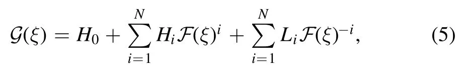
where

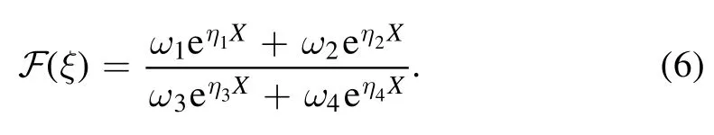
The values of the constants ωi,ηi,(1 ≤i ≤4),H0,Hi,and Li(1 ≤i ≤N) are constant coefficients which need to be obtained.Utilizing the homogeneous balance principle,we can determine the value of N.

· Substituting (5) into (4) with (6) and then collecting all the possible powers ofZj=eηjXfor j=1,…,4 forms an algebraic equation Q(Z1, Z2, Z3, Z4)=0.Comparing the coefficients of Q to zero, one obtains a system of nonlinear equations.

· Eventually,solving the system of nonlinear equations and inserting the obtained solutions into(5)and(6)allows the construction of the exact analytic solutions of (4).

3.Applications of the GERF method

3.1.Applying the GERF method to the (4+1)-dimensional Fokas equation

The prime objective of this work is to obtain the different types of exact soliton solution for a nonlinear Fokas equation and a breaking soliton equation using the GERF method, as mentioned section 2 above.

To simplify nonlinear Fokas equation (1), we assume a wave transformation of the following form:

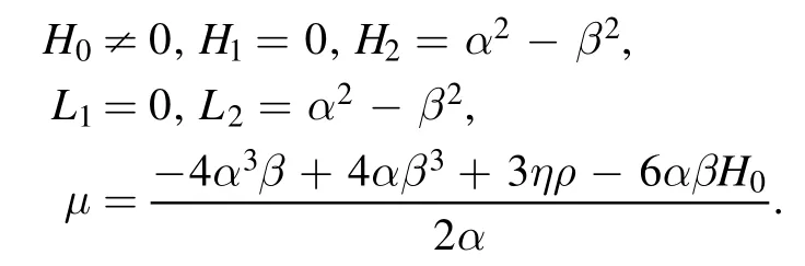
where α, β, μ, ρ, η, and λ are arbitrary constants.Using an expression for μ obtained by substituting (7) into (1), we get an ODE,

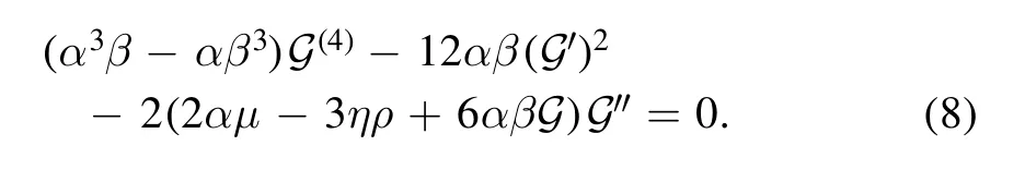
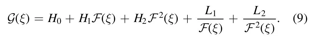
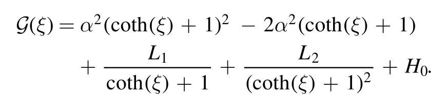
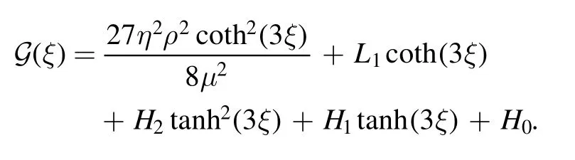
Applying the balancing principle to the termsG(4)and GG′′ of equation (8), gives N+4=N+N+2 which implies N=2.Thus,from(5)we have a trial solution of the following form:

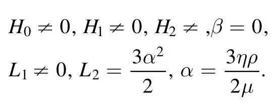
Substituting equation(9)into equation(8)and following the steps of the GERF method, we consider the following cases in order to seek the closed-form solutions of(1)via Mathematica.

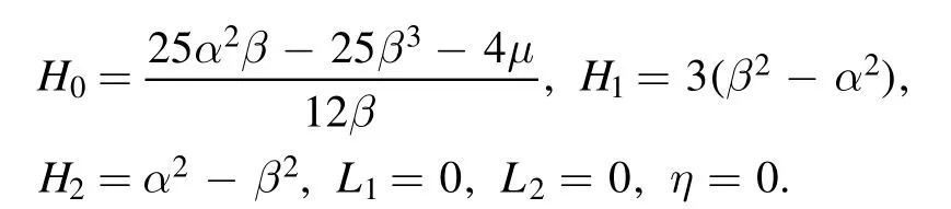
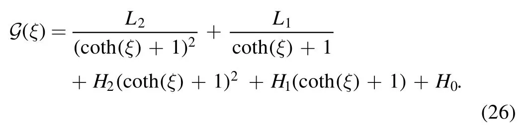
Family 1:For[ω1,ω2,ω3,ω4]=[1,−1,1,1]and[η1,η2,η3, η4]=[1, −1, 1, −1] , equation (6) yields

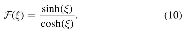
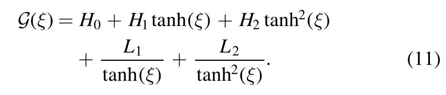
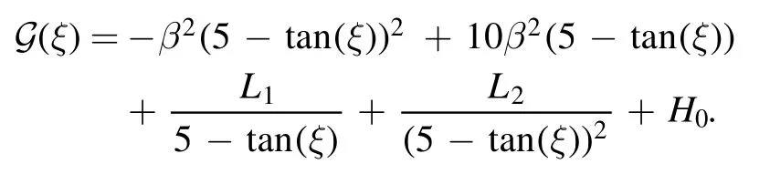
Using (10) and (9), we obtain an expression forG:

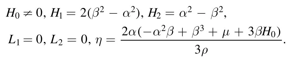
Case 1.1:

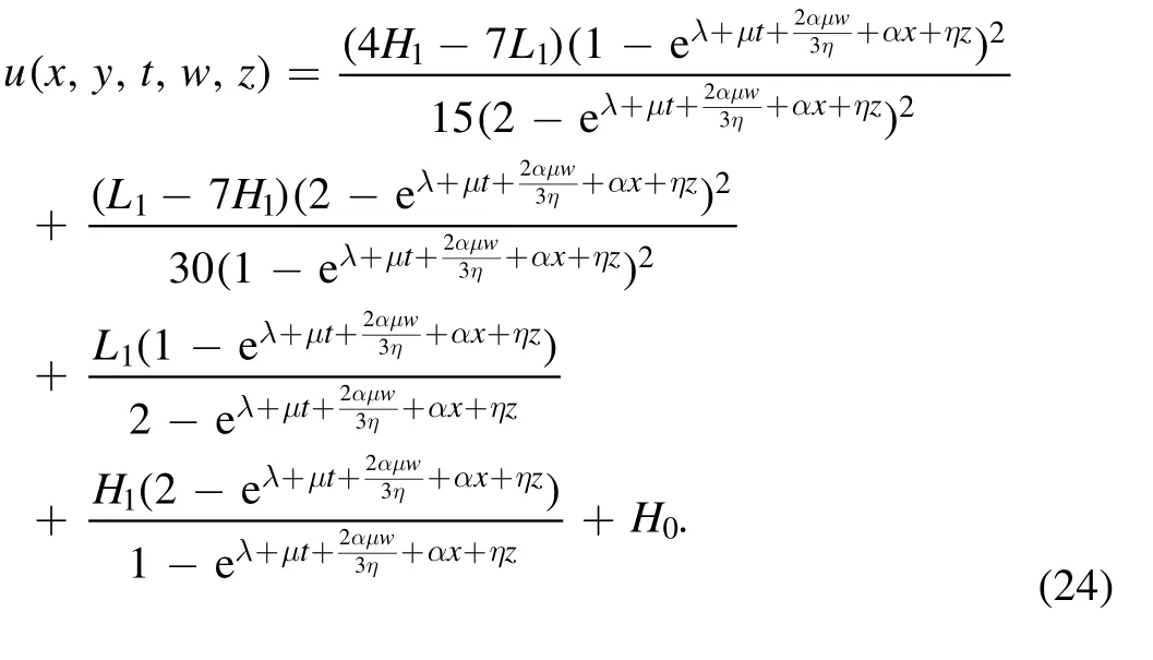
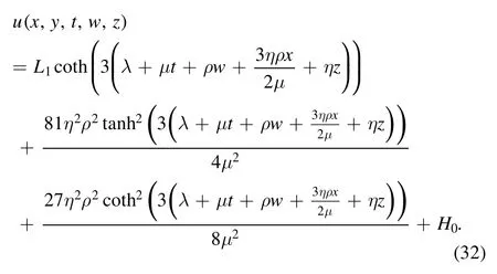
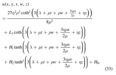
Inserting the values of the constants above into (11),equation (8) then provides

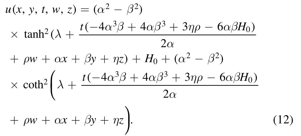
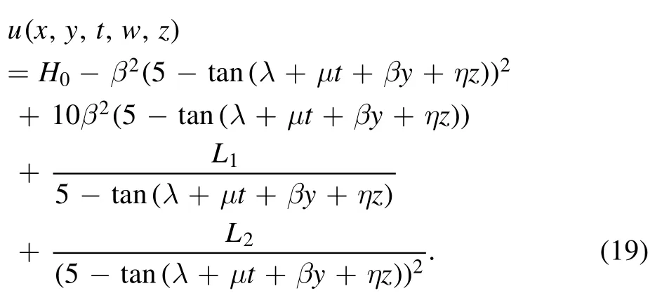
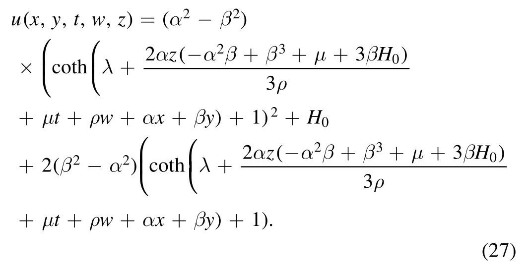
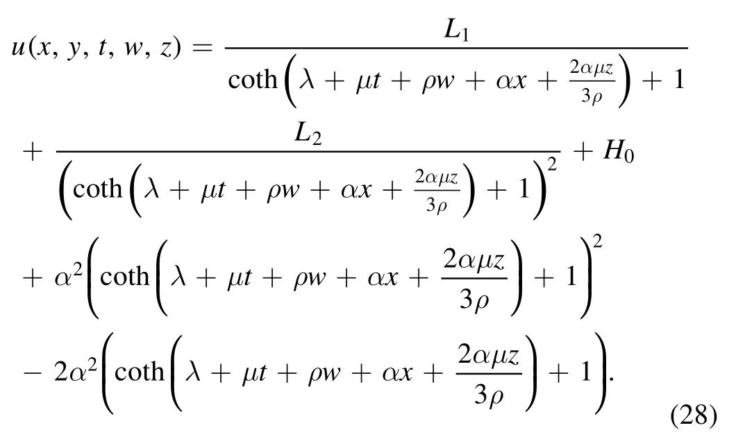
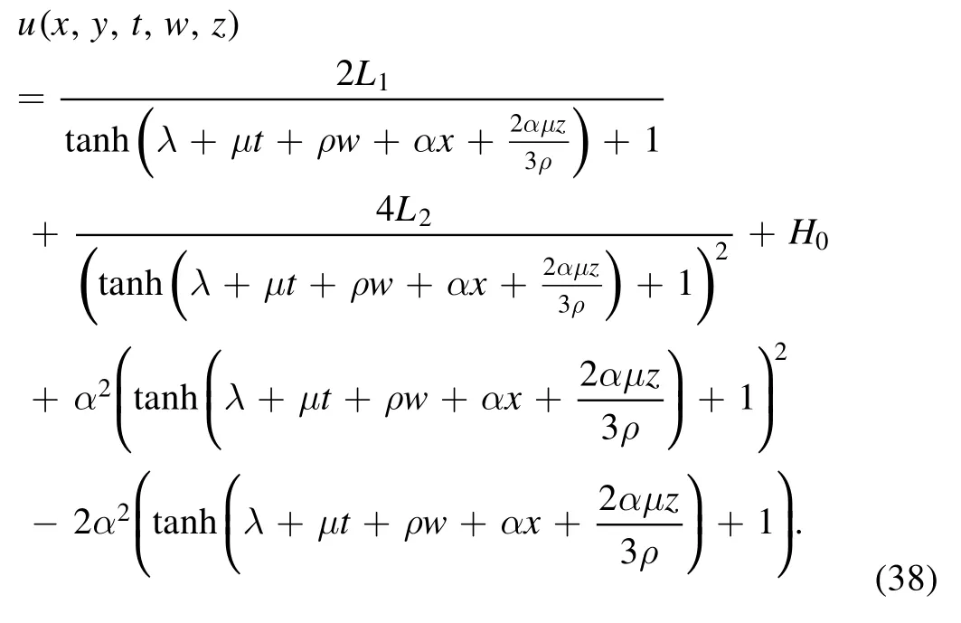
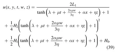
Accordingly, an exact soliton solution of (1) is acquired, as follows:

Case 1.2:

Inserting the values of the constants above into (11),equation (8) then provides:

Accordingly, an exact soliton solution of (1) is acquired as follows:

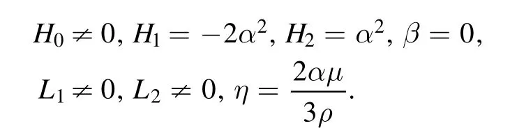
Case 1.3:

Inserting the values of the constants above into (11),equation (8) then provides:

Accordingly, an exact soliton solution of (1) is acquired, as follows:

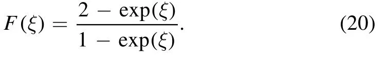
Family 2:For [ω1, ω2, ω3, ω4]=[5 −i, 5+i, 1, 1] and[η1, η2, η3, η4]=[−i, i, −i, i], equation (6) converts into the following form:

Inserting equation(15)into equation(9),we get an expression forG(ξ) in the following form:

Case 2.1:

Inserting the values of the constants above into (16),equation (8) then provides:

Accordingly, an exact soliton solution of (1) is acquired, as follows:

Case 2.2:

Inserting the values of the constants above into (16),equation (8) then provides:

Accordingly, an exact soliton solution of (1) is acquired, as follows:

Case 2.3:

Inserting the values of the constants above into (16),equation (8) then provides:

Accordingly, an exact soliton solution of (1) is acquired, as follows:

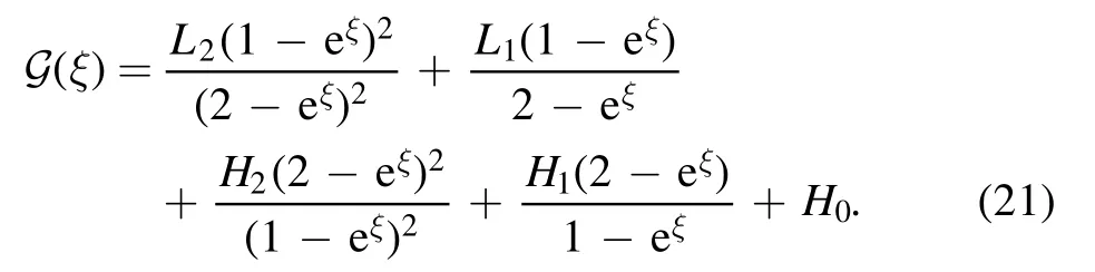
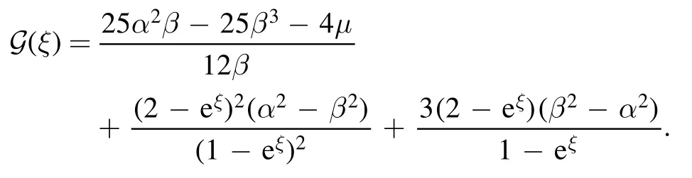
Family 3:For [ω1, ω2, ω3, ω4]=[2, −1, 1, −1] and[η1, η2, η3, η4]=[−1, 0, −1, 0], equation (6) gives:

In view of equations (20) and (9), we have:

Case 3.1:

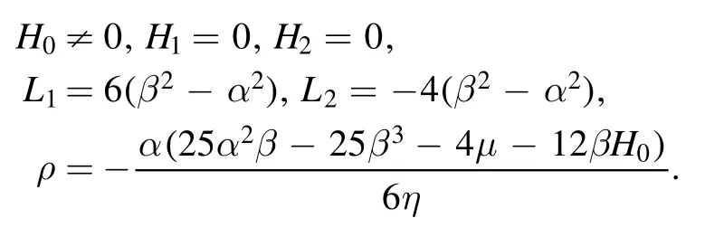
Inserting the values of the above constants into (21),equation (8) then provides:

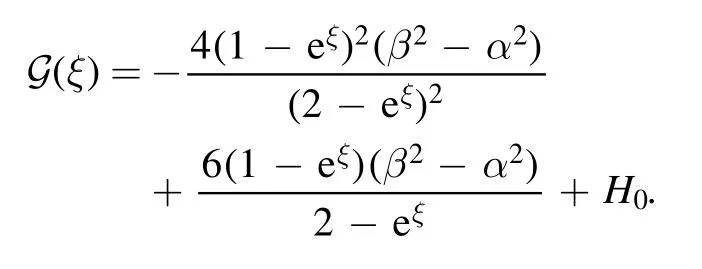
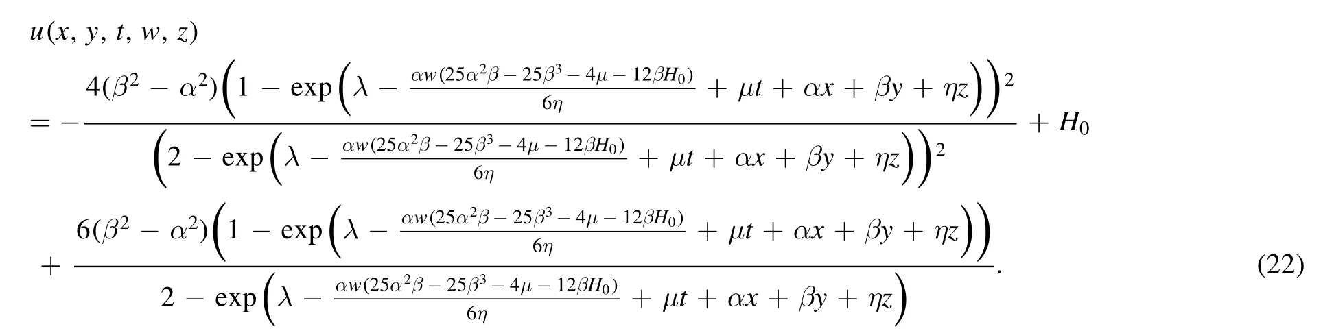
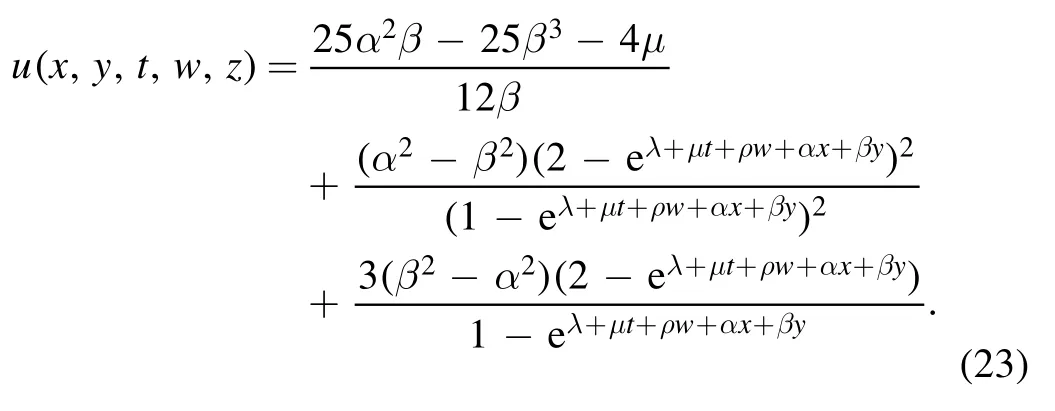
Accordingly, an exact soliton solution of (1) is acquired, as follows:

Case 3.2:

Inserting the values of the above constants into (21),equation (8) then provides:

Accordingly, an exact soliton solution of (1) is acquired, as follows:

Case 3.3:

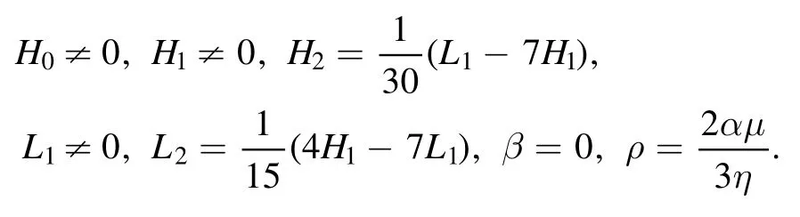
Inserting the values of the above constants into (21),equation (8) then provides:

Accordingly, an exact soliton solution of (1) is acquired, as follows:

Family 4:For[ω1,ω2,ω3,ω4]=[1,1,1,−1]and[η1,η2,η3, η4]=[1, 1, 1, −1], equation (6) gives:

Making use of equations (25) and (9), we get:

Case 4.1:

Inserting the values of the above constants into (26),equation (8) then provides:

Accordingly, an exact soliton solution of (1) is acquired, as follows:

Case 4.2:

Inserting the values of the above constants into (26),equation (8) then provides:

Accordingly, an exact soliton solution of (1) is acquired, as follows:

Case 4.3:

Inserting the values of the above constants into (26),equation (8) then provides:

Accordingly, an exact soliton solution of (1) is acquired, as follows:

Family 5:For[ω1,ω2,ω3,ω4]=[3,−3,3,3]and[η1,η2,η3, η4]=[3, −3, 3, −3], equation (6) gives:

Inserting equation (30) into equation (9), we get:

Case 5.1:

Inserting the values of the above constants into (31),equation (8) then provides:

Accordingly, an exact soliton solution of (1) is acquired, as follows:

Case 5.2:

Inserting the values of the above constants into (31),equation (8) then provides:

Accordingly, an exact soliton solution of (1) is acquired, as follows:

Case 5.3:

Inserting the values of the above constants into (31),equation (8) then provides:

Accordingly, an exact soliton solution of (1) is acquired, as follows:

Family 6:For [ω1, ω2, ω3, ω4]=[2, 0, 2, 2] and [η1, η2,η3, η4]=[2, −2, 2, 0], equation (6) has the form:

Substituting equation (35) into equation (9), we have:

Case 6.1:

Inserting the values of the above constants into (36),equation (8) then provides:

Accordingly, an exact soliton solution of (1) is acquired, as follows:

Case 6.2:

Inserting the values of the above constants into (36),equation (8) then provides:

Accordingly, an exact soliton solution of (1) is acquired, as follows:

Case 6.3:

Inserting the values of the above constants into (36),equation (8) then provides:

Accordingly, an exact soliton solution of (1) is acquired, as follows:

3.2.Applying the GERF method to the (2+1)-D BS equation

We now consider a (2+1)-dimensional BS equation:

To simplify equation (40), we assume a wave transformation of the following form:

where α, β, μand λ are arbitrary constants.Substituting equation(41)into(40),we obtain an ODE of the following form:

By applying the homogeneous balancing principle to the terms G(4)and G ′G ″ in equation (42), we obtain N+4=N+1+N+2, which implies that N=1.Therefore,from equation (5), we obtain a trial solution, as follows:

We substitute equation(43)into(42)and follow the steps of the GERF method.

Family 1:For[ω1,ω2,ω3,ω4]=[−5,7,1,1]and[η1,η2,η3, η4]=[1, 0, 1, 0], equation (6) has the following form:

Substituting (44) into (43), we obtain:

Case 1.1:

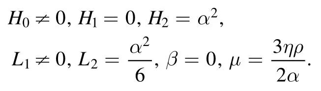
Inserting the values of the above constants into (45),equation (42) then provides:

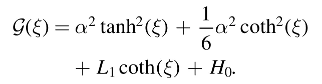
Accordingly, an exact soliton solution of (40) is acquired, as follows:

Case 1.2:

Inserting the values of the above constants into (45),equation (42) then provides:

Accordingly, an exact soliton solution of (40) is acquired, as follows:

Case 1.3:

Inserting the values of the above constants into (45),equation (42) then provides:

Accordingly, an exact soliton solution of BS equation (40) is acquired, as follows:

Family 2:For [ω1, ω2, ω3, ω4]=[3+i, 3 −i, 1, 1] and[η1, η2, η3, η4]=[−i, i, −i, i], equation (6) has the following form:

Substituting (49) into (43), we obtain:

Case 2.1:

Inserting the values of the above constants into (50),equation (42) then provides:

Accordingly, an exact soliton solution of BS equation (40) is acquired, as follows:

Case 2.2:

Inserting the values of the above constants into (50),equation (42) then provides:

Accordingly, an exact soliton solution of BS equation (40) is acquired, as follows:

Case 2.3:

Inserting the values of the above constants into (50),equation (42) then provides:

Accordingly, an exact soliton solution of BS equation (40) is acquired, as follows:

Family 3:For [ω1, ω2, ω3, ω4]=[7 −i, −7 −i, −1, 1]and[η1,η2,η3,η4]=[i,−i,i,−i],equation (6)has the form

Substituting (54) into (43), we obtain:

Case 3.1:

Inserting the values of the above constants into (55),equation (42) then provides:

Accordingly, an exact soliton solution of BS equation (40) is acquired, as follows:

Case 3.2:

Inserting the values of the above constants into (55),equation (42) then provides:

Accordingly, an exact soliton solution of BS equation (40) is acquired, as follows:

Case 3.3:

Inserting the values of the above constants into (55),equation (42) then provides:

Accordingly, an exact soliton solution of BS equation (40) is acquired, as follows:

Family 4:For [ω1, ω2, ω3, ω4]=[4, 0, 4, 4] and [η1, η2,η3, η4]=[4, −4, 4, 0], equation (6) has the following form:

Substituting (59) into (43), we have,

Case 4.1:

Inserting the values of the above constants into (60),equation (42) then provides:

Accordingly, an exact soliton solution of BS equation (40) is acquired, as follows:

Case 4.2:

Inserting the values of the above constants into (60),equation (42) then provides:

Accordingly, an exact soliton solution of BS equation (40) is acquired, as follows:

Case 4.3:

Inserting the values of the above constants into (60),equation (42) then provides:

Accordingly, an exact soliton solution of BS equation (40) is acquired, as follows:

Family 5:For [ω1, ω2, ω3, ω4]=[1+i, 1 −i, 2, 2] and[η1, η2, η3, η4]=[i, −i, i, −i], equation (6) has the following form:

Substituting (64) into (43), we obtain:

Case 5.1:

Inserting the values of the above constants into (65),equation (42) then provides:

Accordingly, an exact soliton solution of BS equation (40) is acquired, as follows:

Case 5.2:

Inserting the values of the above constants into (65),equation (42) then provides:

Accordingly, an exact soliton solution of BS equation (40) is acquired, as follows:

Family 6:For [ω1, ω2, ω3, ω4]=[2i, 2i, i, i] and [η1, η2,η3, η4]=[0, 0, −7, 0], equation (6) has the following form:

Substituting (68) into (43), we obtain:

Case 6.1:

Inserting the values of the above constants into (69),equation (42) then provides:

Accordingly, an exact soliton solution of BS equation (40) is acquired, as follows:

Case 6.2:

Inserting the values of the above constants into (69),equation (42) then provides:

Accordingly, an exact soliton solution of BS equation (40) is acquired, as follows:

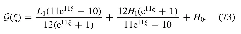
Family 7:For [ω1, ω2, ω3, ω4]=[−12, −12, −11, 10]and [η1, η2, η3, η4]=[10, −1, 10, −1], equation (6) has the following form:

Substituting (72) into (43), we obtain:

Case 7.1:

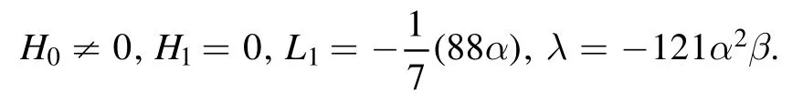
Inserting the values of the above constants into (73),equation (42) then provides:

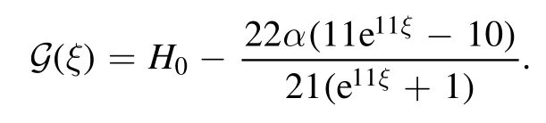
Accordingly, an exact soliton solution of BS equation (40) is acquired, as follows:

Case 7.2:

Inserting the values of the above constants into (73),equation (42) then provides:

Accordingly,an exact soliton solution of BS(40)is acquired,as follows:

Case 7.3:

Inserting the values of the above constants into (73),equation (42) then provides:

Accordingly, an exact soliton solution of BS equation (40) is acquired, as follows:

4.Physical interpretation of the obtained solutions

The dynamical and physical behaviors of the analytic wave solutions of the nonlinear partial differential equations are always preferable for an accurate understanding of the behavior of these solutions.In this section,we aim to discuss the physical behaviors of our newly established exact soliton solutions,singular solutions that include hyperbolic functions,rational form solutions, trigonometric functions, and exponential rational functions, using the best suitable choices of arbitrary constants in appropriate ranges by employing the computational tool Mathematica.Figures 1–7 depict the dynamics of some well-known solutions in the form of soliton solutions,bell-shaped solitons,triple solitons,combo singular solitons, breather-type waves, singular kink-shaped solitons,and novel solitary waves.The dynamics of exact soliton solutions are intensively analyzed, as follows:

Figure 1 depicts two different dynamical shapes for equations(13)with 1(a),showing singular solitons formed for the parameters α=0.25,η=0.1,ρ=17,λ=1.9,and H0=3 for the ranges of −2000 ≤x ≤2000 and −2000 ≤z ≤2000 at t=−5, w=0.3, while 1(b) represents the singular double soliton wave profile for the values α=0.25, η=0.1, ρ=16,λ=1.9, and H0=3 for the ranges −2000 ≤x ≤2000 and−2000 ≤z ≤1900 at t=3 and w=0.2.

Figure 1.Two distinct dynamical shapes for equation(13)show singular solitary wave profiles for the values:(a)α=0.25,η=0.1,ρ=17,λ=1.9, and H0=3; (b)α=0.25, η=0.1, ρ=16, λ=1.9, and H0=3.

Figure 2 shows the two distinct dynamical shapes of equation (23), in which 2(a) depicts the singular soliton wave profile formed with a kink for suitable constant values α=0.5,β=5, ρ=16, λ=45, and μ=1, for the ranges of −5000 ≤x ≤7000 and −3000 ≤y ≤3000 at t=−5, w=0.4; 2(b)represents double soliton wave profiles with a kink wave for the values α=0.5,β=5,ρ=16,λ=45,and μ=1 for the ranges of −6000 ≤x ≤4000 and −3000 ≤x ≤3000 at t=−5 and w=0.5.

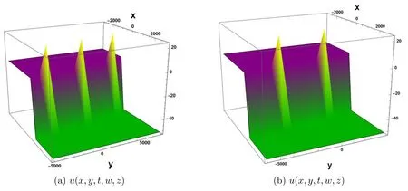
Figure 2.Two distinct dynamical shapes for equation(23)show singular solitary wave profiles with kink waves for the values:(a)α=0.5,β=5, ρ=16, λ=45, and μ=1; (b) α=0.5, β=5, ρ=16, λ=45, and μ=1.

Figure 3 depicts the shapes of bell-shaped singular solitons for equation (27), in which 3(a) takes the different parameter values α=0.5, β=5, η=0.1, ρ=16, λ=45, μ=1, and H0=2, for the ranges of −4000 ≤x ≤7000 and−3000 ≤z ≤3000 at t=−1, w=0.5, y=0.1 and the 3(b)profile takes the values α=0.3,β=5,η=0.1, ρ=20,λ=50,μ=1, and H0=2 for the ranges of −3000 ≤x ≤3000 and−5000 ≤z ≤5000 at t=−1, w=0.5, and y=0.5.

Figure 3.Two distinct dynamical shapes of singular soliton profiles for equation (27): (a) for the values α=0.5, β=5, η=0.1, ρ=16,λ=45, μ=1, and H0=2; (b) for the values α=0.3, β=5, η=0.1, ρ=20, λ=50, μ=1, and H0=2.

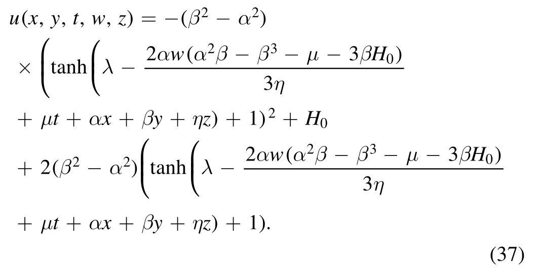
Figure 4 shows two different shapes of bell-shaped soliton for equation (37), in which 4(a) represents the singlesoliton profile for the values α=−0.25, β=−0.5, η=0.2,μ=1600, λ=0, and H0=0.3, for the ranges of −4000 ≤x ≤2000 and −1000 ≤z ≤1000 at t=−0.2, w=0.2, and y=0.5 and figure 4(b) represents the double solitons for the values α=−0.35, β=−0.1, η=0.2, μ=1500, λ=0, and H0=1000 for the ranges of −2000 ≤x ≤4000 and −500 ≤z ≤1000 at t=−0.2, w=0.2, and y=0.5.

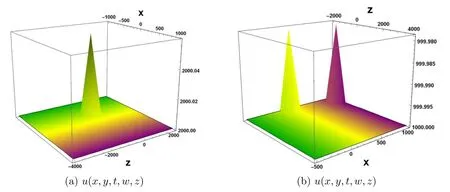
Figure 4.Two distinct dynamical shapes for equation (37) show singular bell-shaped soliton wave profiles for the values: (a)α=−0.25,β=−0.5, η=0.2, μ=1600, λ=0, and H0=0.3; (b)α=−0.35, β=−0.1, η=0.2, μ=1500, λ=0, and H0=1000.

Figure 5 shows the four different three-dimensional profiles of equation (46), which represent the interactions of solitons with kink waves for different values of constants in the ranges of −60000 ≤x ≤60000 and −5000 ≤y ≤7000,5(a)α=−0.4, β=1.5 λ=−1.7, and H0=0.3 at t=−2.5;5(b)α=−0.35,β=1.5,λ=−1.5,and H0=1.9 at t=−15;5(c)α=−0.55, β=1.5, λ=−1.5, and H0=0.1 at t=2.5 and 5(d)α=−0.35, β=1.5, λ=−1.5, and H0=0.3 at t=−2.5.Based on the numerical simulation,we confirm that the four dynamical structures of the acquired exact soliton solutions are also useful for analyzing the interactions between diverse solitons with kink waves.

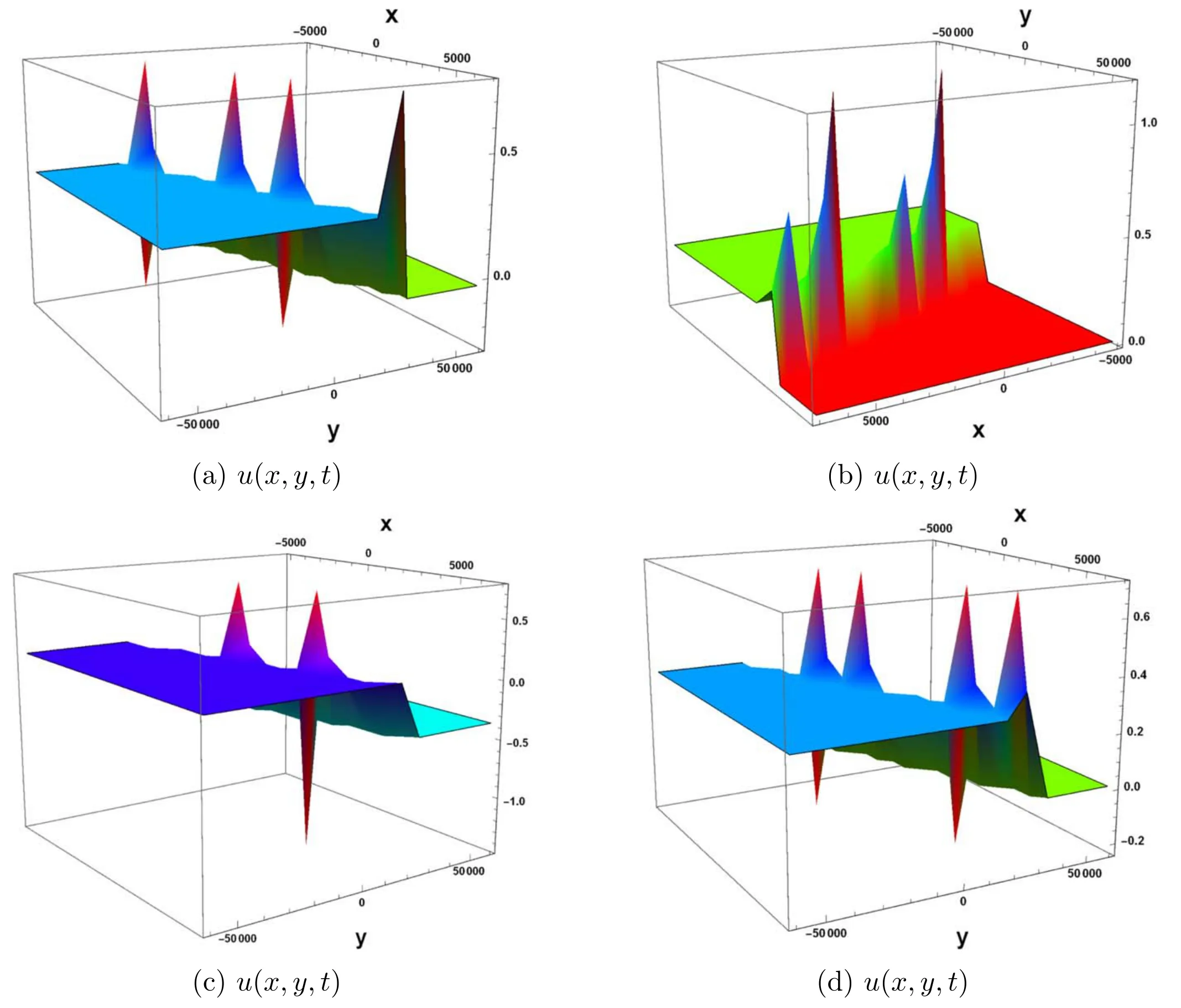
Figure 5.Four distinct dynamical shapes for equation (46) show the interaction of solitary wave solutions with singular kink waves for the values: (a)α=−0.4, β=1.5, λ=−1.7, and H0=0.3 at t=−2.5; (b)α=−0.35, β=1.5, λ=−1.5, and H0=1.9 at t=−15;(c)α=−0.55, β=1.5, λ=−1.5, and H0=0.1 at t=2.5; (d)α=−0.35, β=1.5, λ=−1.5, and H0=0.3.

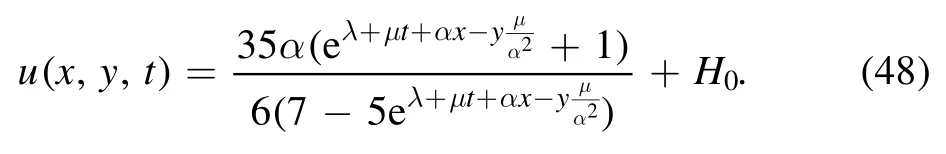
Figure 6 depicts the interaction of solitons and kink waves for equation (48), in which 6(a) represents triple solitons with kink waves for the values α=−0.25, μ=1.5,λ=−1.5, and H0=0.3, for the ranges of −40000 ≤x ≤50 000 and −1000 ≤y ≤1000 at t=5 and 6(b) shows double solitons with a kink wave profile for the values α=−0.25, μ=2.5, λ=−1.5, and H0=0.1 for the ranges of −60000 ≤x ≤60 000 and −1000 ≤x ≤1000 at t=−5.We confirm that the dynamics of the aforementioned closed-form solutions can be used to investigate the interactions of various solitons with kink waves.

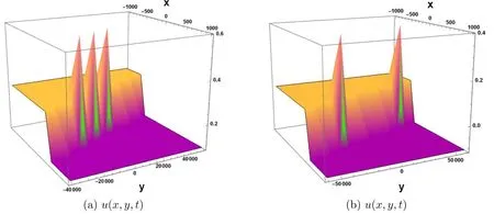
Figure 6.Two distinct dynamical shapes for equation (48) show the interaction between solitons and kink waves for the values:(a)α=−0.25, μ=1.5, λ=−1.5, and H0=0.3; (b)α=−0.25, μ=2.5, λ=−1.5, and H0=0.1.

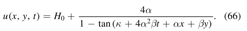
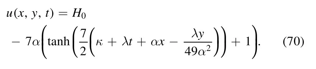
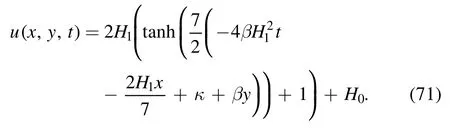
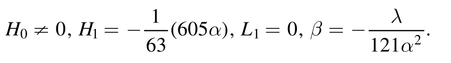
Figure 7 shows two distinct dynamical shapes for equation (74) that demonstrate the interaction between solitons and kink waves for the values: (a)α=0.5, β=5, κ=0.1, and H0=2 for the ranges of −4000 ≤x ≤4000 and −1000 ≤y ≤1000 at t=−5; (b)α=0.9, β=5, κ=0.1, and H0=2 for the ranges of −1000 ≤x ≤1000 and −1000 ≤y ≤3000 at t=0.0125.

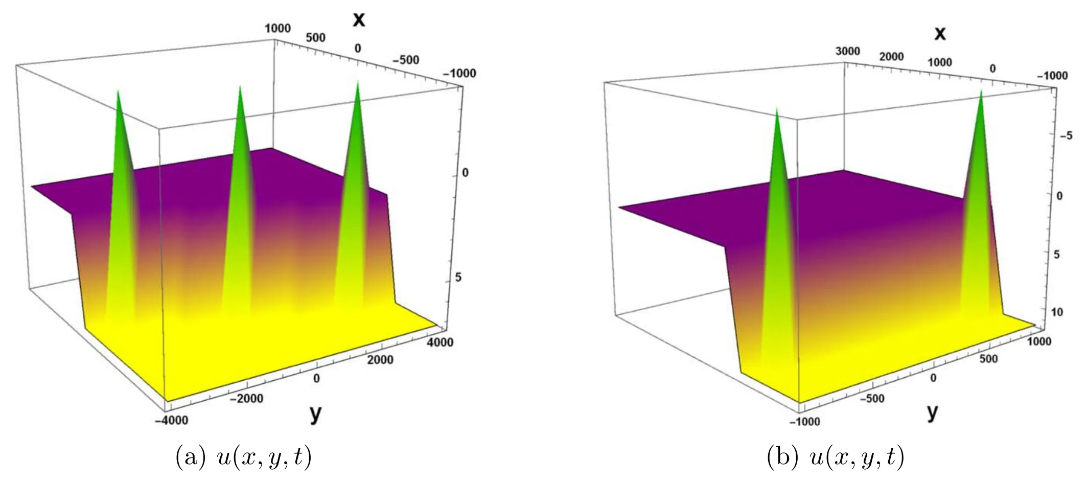
Figure 7.Two distinct dynamical shapes for equation(74)depict the interaction between solitons and kink waves for the values:(a)α=0.5,β=5, κ=0.1, and H0=2; (b)α=0.9, β=5, κ=0.1, and H0=2.

It has been shown that the newly established solutions of the higher-dimensional Fokas equation and the (2+1)-dimensional BS equation obtained using the current proposed method(which is a generalized exponential rational function technique)differ from the works of other authors, who have commonly used the analytic techniques reported in [38–43, 47–50].The solutions we obtained in this study are completely novel and more generalized exact solutions than the previous results.

5.Conclusions

In summary, we have studied two different NLEEs, namely the Fokas equation in (4+1)-dimensions and the breaking soliton equation in (2+1)-dimensions by utilizing the GERF method.We have successfully obtained numerous exact soliton solutions,such as single solitons,double solitons,triple solitons,quadruple solitons, elastic interaction solutions between quintuple solitons with kink-waves, localized solitary waves, and rational function solutions.To the best of our knowledge, all of the constructed closed-form solutions are completely novel and have never been reported in the literature.The solutions obtained are very useful for understanding the dynamical behaviors of the physical phenomena of these complex models.The dynamical structures of some exact-solitary wave solutions were also demonstrated graphically by assigning suitable values to the free parameters,which helps to interpret the physical behaviors of these dynamical models.All the newly formed solutions to the Fokas equation and the BS equation have a wide range of applications in areas of nonlinear sciences such as plasma physics, optical engineering, oceanography engineering, fluid dynamics, nonlinear dynamics, condensed-matter physics, and many other associated fields of engineering physics and the mathematical sciences.Generally, solitary wave solutions provide justification and additional explanation for dispersion management strategies.Furthermore, the dynamical behaviour of solitary wave profiles suggests the existence of an overarching theory for estimating the effects of multiplexing in many physical systems.The computerized symbolic work and extracted solutions show that the current method is effective, robust, and straightforward.Many other NLEEs can be solved using the efficient GERF method.

Acknowledgments

This work is funded by the Science and Engineering Research Board, SERB-DST, India, under project scheme MATRICS(MTR/2020/000531).The author,Sachin Kumar,has received this research grant.

ORCID iDs