Bright, periodic, compacton and bell-shape soliton solutions of the extended QZK and(3 + 1)-dimensional ZK equations

M Ali Akbar, Md Abdul Kayum,2 and M S Osman

1 Department of Applied Mathematics, University of Rajshahi, Bangladesh

2 Department of Computer Science & Engineering, North Bengal International University, Rajshahi,Bangladesh

3 Department of Mathematics, Faculty of Science, Cairo University, Giza 12613, Egypt

Abstract The(3 + 1)-dimensional Zakharov–Kuznetsov(ZK)and the new extended quantum ZK equations are functional to decipher the dense quantum plasma, ion-acoustic waves, electron thermal energy,ion plasma,quantum acoustic waves,and quantum Langmuir waves.The enhanced modified simple equation (EMSE) method is a substantial approach to determine competent solutions and in this article, we have constructed standard, illustrative, rich structured and further comprehensive soliton solutions via this method.The solutions are ascertained as the integration of exponential,hyperbolic,trigonometric and rational functions and formulate the bright solitons, periodic, compacton, bellshape, parabolic shape, singular periodic, plane shape and some new type of solitons.It is worth noting that the wave profile varies as the physical and subsidiary parameters change.The standard and advanced soliton solutions may be useful to assist in describing the physical phenomena previously mentioned.To open out the inward structure of the tangible incidents,we have portrayed the three-dimensional,contour plot,and two-dimensional graphs for different parametric values.The attained results demonstrate the EMSE technique for extracting soliton solutions to nonlinear evolution equations is efficient, compatible and reliable in nonlinear science and engineering.

Keywords: (3 + 1)-dimensional ZK, the extended QZK equation, enhanced modified simple equation method, soliton solutions, NLEEs

1.Introduction

Nonlinear evolution equations (NLEEs) play a very important role in describing many physical features, particularly in quantum acoustic waves, quantum Langmuir waves, dense quantum plasma, ion-acoustic waves, electron thermal energy,ion plasma,solid state physics,optical fibers,chemical physics,chaos theory, mathematical physics, astrophysics, biophysics,nuclear physics, fluid mechanics, engineering problems [1, 2]etc.Nonlinear soliton solutions of these NLEEs play a fundamental role in unraveling the dynamics and describing the facts.Thus, different methods are used to search soliton solutions to these NLEEs.Some of them are the extended simple equation technique [3], the generalized Kudryashov technique [4], the first-integral technique[5],the new auxiliary equation technique[6], the Bernoulli sub-equation function technique [7, 8], the Riccati–Bernoulli sub-ODE method [9–11], the sine-Gordon expansion technique[12,13],the sine–cosine technique[14],the generalized unified technique[15],the modified Khater method[16], the tanh–coth method [17], He’s variational principle[18, 19], the Bcklund transformation method [20], the unifeid Riccati equation expansion method [21], the extended Kudryashov method [22], the improved(G′/G) -expansion method[23], the functional variable method [24], the exp-expansion technique [25], the improvedF-expansion technique [26], the MSE technique [27–30], the enhanced MSE method [31], the Jacobi elliptic functions method [32–35], and other different techniques [36–40].

In various fields of physics, applied mathematics, and engineering, the Zakharov–Kuznetsov (ZK)equation is used.The new extended quantum ZK (QZK) and the (3 + 1)-dimensional ZK equations were derived for finite but small amplitude ion-acoustic waves in a quantum magneto-plasma by using the reductive perturbation theory and the quantum hydrodynamical model [41].In this study, we consider the enhanced MSE technique to search bright solitons, periodic,compacton, bell-shape, parabolic, singular periodic and other general soliton solutions of the (3 + 1)-dimensional ZK equation and the new extended quantum QZK equation [42].The ZK equation is one of the two canonical two-dimensional extensions of the Korteweg–de Vries equation, which was initially developed in two dimensions for weakly nonlinear ion-acoustic waves in strongly magnetized lossless plasma.The new extended QZK equation [43] is:

wherev(x,y,t)represents the electrostatic wave potential with the temporal variabletand spatial variablesx,yandα,β,γare all constants.The coefficients ofβandγdescribe the multi-dimensional dispersion terms,the coefficient ofαis the nonlinear term,andvtis the evolution with respect to time.

In the subsequent, we consider the (3 + 1)-dimensional ZK [44]:

where α is the nonlinear coefficient andβ,γ,δare the dispersion coefficients.In[44], the ZK equation was derived by putting in use the reductive perturbation technique and the quantum hydrodynamic model and some periodic, explosive,and solitary wave solutions are obtained with the help of the extended Conte’s truncation technique.

The exact solutions and symmetry reductions to the extended QZK equation have been derived by Lie symmetry analysis in[45].In[46],the optimal system and conservation law were used for further investigation of the extended QZK equation.To obtain the exact travelling wave solutions to the extended QZK equation, El-Ganaini and Akbar [47] contrive the modified simplest equation technique, the extended simplest equation technique,and the simplest equation technique.Baskonus et al [48] extracted hyperbolic and complex function solutions of the extended QZK equation by using the sine-Gordon expansion technique.Raza et al [49] used the trial equation method to search soliton and periodic solutions of equation (1).

The multiple soliton solutions and new exact solitary wave solutions of (2) were attained by means of the Hirota’s bilinear technique and the auxiliary equation method in [50].Ebadi et al[51]used the adaptedF-expansion technique,expfunction technique, and the(G′/G) -expansion technique to find exact travelling wave solutions.Bhrawy et al [52] introduced the extendedF-expansion technique for finding the complexiton solutions, singular soliton, non-topological, and topological solutions.In[53],the authors applied the extended generalized(G′/G)-expansion technique to determine new exact solutions of (2).Lu et al [54] introduced the modified extended direct algebraic method to extract the elliptic function solutions,soliton and new exact solitary wave solutions of(2).New types of travelling wave solutions of(2)were attained by applying the generalized(G′/G)-expansion technique and the improved tan (φ/2) -expansion technique in [55].Zayed et al[56] applied the(G′/G, 1/G)-expansion method to extract further exact solutions of (2).Recently, Vinita and Ray [57]used the Lie symmetry analysis to study the equation (2) and new exact solitary wave solutions are attained and also derived the conservation laws to the QZK equation.

The enhanced modified simple equation(EMSE)method is recently developed a significant approach to determining competent solutions that is effective,compatible,and reliable to extract soliton solutions to NLEEs.This method have been used to examine the (1 + 1)-dimensional Burgers–Fisher equation with variable coefficients, the (2 + 1)-dimensional ZK equation with variable coefficient,the FitzHugh–Nagumo equation, the Burgers–Huxley equation [58], the modified Volterra equations,the Burger–Fisher equation[59],the Phi-4 equation [60], Chafee–Infante equation [61], the Gardner equation and the modified Benjamin–Bona–Mahony equation

[62].The (3 + 1)-dimensional ZK and the new extended QZK equations are important mathematical models to decipher ion-acoustic waves, quantum acoustic waves, quantum Langmuir waves, etc.To the optimal of our cognition and based on the analysis of the documents reachable in the literature obtained, the formerly introduced equations have not been investigated by the EMSE technique earlier.Thus,supported by the earlier studies, the aim of this article is to ascertain standard, realistic and far-reaching compatible solutions to these equations through the EMSE method.The feature of the solutions is that they extract bright solitons,periodic, compacton, bell-shape, parabolic shape, singular periodic and other solitons for certain values of the associated parameters.

The remaining of the article is sorted out as follows: the explanation of the enhanced MSE technique is given in section 2.In section 3, we use technique to search the advanced and wide-spectral soliton solutions.Some of the important graphical depictions of the solutions obtained are given in section 4.Finally in the last section,the conclusion is given.

2.The EMSE technique

In this section, we concisely explain the EMSE technique[58–62].Let us consider a general NLEE in the subsequent form:

whereL is a polynomial with respect to the wave functionv(x,y,z,t)in which the highest order derivatives and nonlinear terms are involved.The following are the basic steps of this technique:

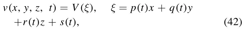
Step 1.The wave variableξ=p(t)x+q(t)y+r(t)z+s(t),wherev(x,y,z,t)=V(ξ)remodels equation (3) into a nonlinear differential equation in the follow way:

whereV=V(ξ), dot specifies the differentiation related to timet, and prime (′) specifies the differentiation with respect toξ.

Step 2.The solution of the reduced equation(4),in agreement with the EMSE method can be put into the form:

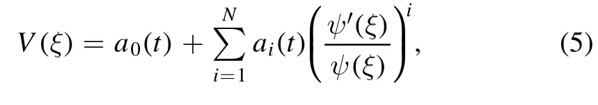
wherea0(t),a1(t),a2(t),…,aN(t)are the unknown function of‘t’ to be evaluated, such thataN(t) ≠0,andψ′(ξ)≠0.The outstanding feature of this approach is that, instead of constants, the coefficients ofψ(ξ)-iare the function oft, andψ(ξ)is an unknown function or not a solution of any wellknown equation.

Step 3.The balancing theory between the nonlinear and linear terms appearing in equation (4), results the balance numberNarise in solution (5).

Step 4.Using the solution (5) and its necessary derivatives into equation(4),together with the balance numberN,yield a polynomial ofψ(ξ)-i, wherei= 1,2,3,…,N.Collecting all the terms of same power and equating them to zero, it is attained a system of differential and algebraic equations, can be estimated to finda0,ai,p,q,r,sandψ(ξ).Thus, we can establish inclusive,fresh and standard soliton solutions of(3)by substituting the above values into the solution (5).

3.Solutions analysis

In this section, bright solitons, periodic, compacton, parabolic, bell-shape, singular periodic and other types of soliton solutions of the (3 + 1)-dimensional ZK and the new extended QZK equations are established via the enhanced MSE technique.

3.1.The new extended QZK equation

In this section,we derive the general solitary wave solution in terms of hyperbolic function, trigonometric function, exponential function and rational function of the new extended QZK equation using the enhance MSE technique.The wave transformation

remodel the equation (1) into the subsequent equation:

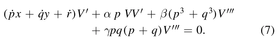
We attain equation (8) after integrating (7),

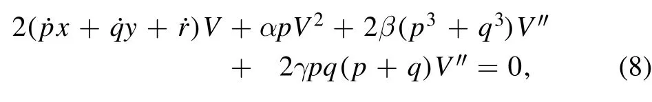
setting the zero-integrating constant.

Using the balancing principle betweenV″ and V2, we obtainN= 2.

Therefore, the equation (8) has a solution of the following form

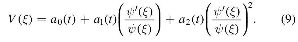
Inserting solution (9) and its necessary derivatives into equation(8);equating all the coefficients ofψ-i,xψ-i,yψ-i,i=0, 1,2,3,4, and setting them to zero, we attain the algebraic and differential equations as follows:

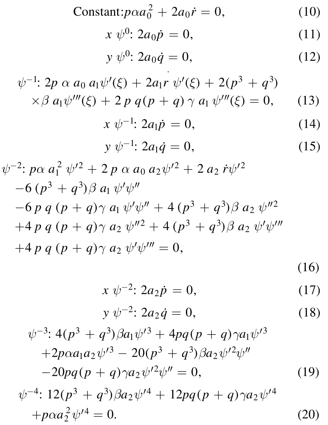
Equations (11), (12), (14), (15), (17) and (18) give the subsequent results:

=0 and= 0.Thus,p=handq=k,wherehandkare integrating constants.

On the other hand, from equations (10) and (20), we found

a0(t) =0,-2r˙/hαanda2(t) =sincea2(t) ≠0.

Equation (19) provides the subsequent result:

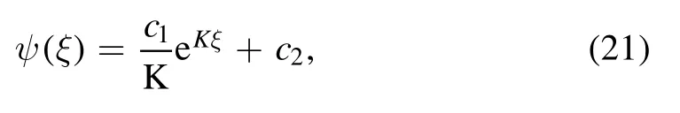
wherec1,c2are constants of integration andK=

The following cases should now be discussed:

Case 1.Whena0=0.

Inserting the values ofψ(ξ),a2(t)anda0(t)into(13),we obtain

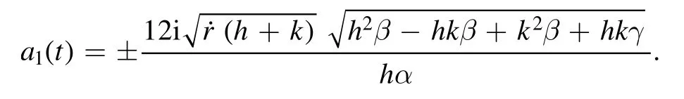
Since the values ofp,q,a0,a1,a2andψsatisfy equation(16),the values ofp,q,a0,a1,a2andψare admissible to determine the soliton solutions.

Using the values ofa0,a1,a2andψ(ξ)into the solution(9), we ascertain

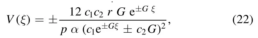
By using the transformation between the exponential and hyperbolic functions, solution (22) is reduced to the subsequent soliton solution:

Choosing the value of arbitrary constants, c1= ±4 andtherefore, we attain

whereξ=hx+ky+r(t).

Again, choosingc1= ±12andthe solution(23) turns to be

Moreover, if we assign,c1= ±G,c2= ±1orc1= ±1,we obtain the succeeding hyperbolic function solutions of equation (8)

Thus,subject to the spatio-temporal coordinates,we attain the subsequent bright and singular soliton to the extended QZK equation as

We attain the subsequent trigonometric function solutions, from solutions (28) and (29):

Case 2.When.

Introducing the values ofa0(t),a2(t)andψ(ξ)into(13),yields

Substituting the values ofa0,a1,a2andψ(ξ)into (9), we attain the ensuing solution

The solution (32) can be written as

Setting the valuesc1= ±6and of the arbitrary constants in (33), we extract

whereξ=h x+k y+r(t).

Yet again, settingc1= ±18andwe obtain

Alternatively, if we setc1= ±H,c2= ±1orc1= ±1,we ascertain the under mentioned soliton solutions

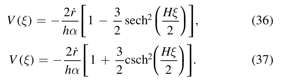
Subject to the temporal-spatial coordinates, we obtain the interpreted bright and singular soliton to the extended QZK equation as follows:

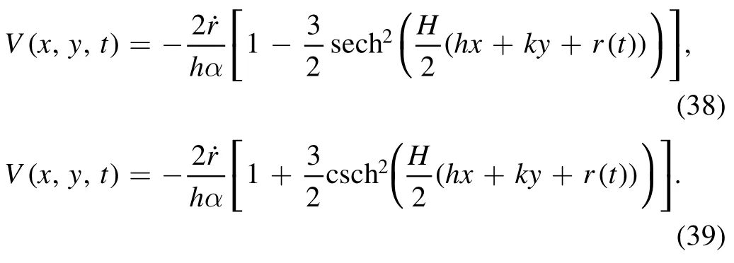
The periodic soliton for solutions (38) and (39) is considered to be:

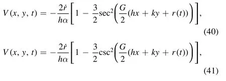
whereGis provided in the above.The solutions (28)–(31)and (38)–(41) represent bright, parabolic soliton, bell-shape soliton, singular periodic soliton, and compacton.

3.2.The (3 + 1)-dimensional ZK equation

In this section, relating to exponential function, rational function, hyperbolic function and trigonometric function, we obtain the general solitary wave solution to the (3 + 1)-dimensional ZK equation via the EMSE method.The wave variable

reduces the (3 + 1)-dimensional ZK equation (2) into the ensuing equation:

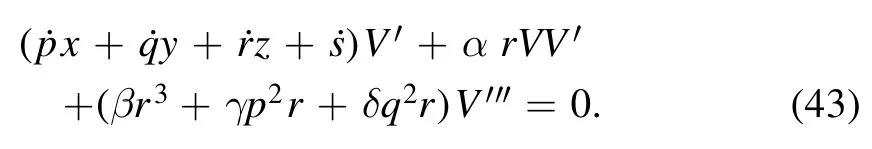
Integrating (43) with zero integrating constant, we obtain

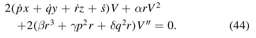
Applying the balance principle between the nonlinear termV2and highest order derivativeV″ , we foundN= 2.

Thus, the solution of equation (44) accept the following form

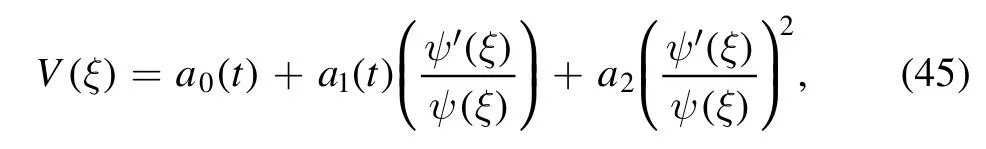
wherea0,a1anda2are an unknown function oft,andψ′(ξ)≠0.

Putting the values ofV(ξ)and it’s twice derivative into(44)and equalizing the coefficients of same power to zero,we attain some algebraic and differential equations as follows:

From equations (47)–(49), (51)–(53) and (55)–(57), it is found

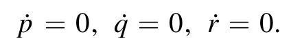
Integrating the above expressions with respect to time, yields

where l, m and n are the constants of integration.

Equation (58) gives the following result:

wherec3andc4are constants of integration andK′=.

Solving equations(46)and(59)and putting the values ofp,q,r, we attain

Case 1.Whena0=0,

Using the values ofa0,a2,ψinto the equation (50) and solving fora1, we acquire

Inasmuch as equation(54)is satisfied for the values ofp,q,r,a0,a1,a2andψ, these values are acceptable for determining the soliton solutions.

Substituting the values ofa0,a1,a2andψinto the solution (45), we attain the subsequent exponential function solution

Transforming the exponential function solution (61) into the hyperbolic function solution, we attain

Sincec3andc4are integral constants,their values could be set at random.As a result,we can choose the values ofc3andc4arbitrarily.Therefore, if we choosec3= ±5 /2andc4= ±1 /2M,the solution (62) turns out to be

Again, if we choosec3= ±M,c4= ±1orc3= ±1,we attain the hyperbolic function solutions of equation (44) in the ensuing

Thus, the bell-shape and singular solitons to the (3 + 1)-dimensional ZK equation in relation to the space-time coordinates are

In relation to (66) and (67), the trigonometric function solutions can be simulated as:

.

Case 2.When.

Embedding the values ofa0,a2,ψinto (50) and deciphering fora1, yield

For these values ofa0,a1,a2andψ, from solution (45), we attain

The solution (70) of the exponential function can be formulated as

For the valuesc3= ±6andsolution (71) turns to the soliton solutions:

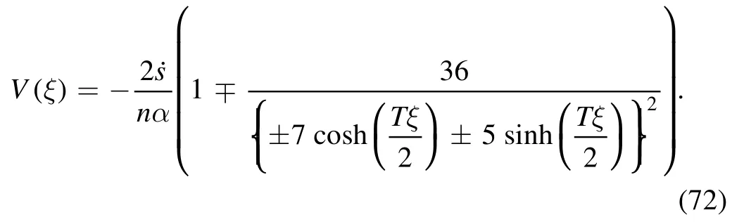
Furthermore, if we setc3= ±T,c4= ±1orc3= ±1,solution (72) turns into:

Therefore, we attain the under mentioned bell-shape and singular soliton solutions subject to space-time coordinates.

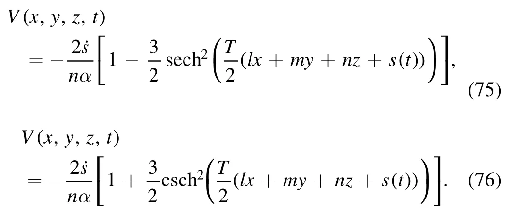
Relating to(75)and(76),the trigonometric function solutions can be constructed as:

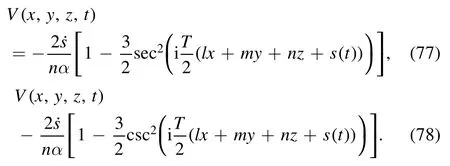
The solutions (66)–(69) and (75)–(78) produce the bright,periodic, singular bell-shaped and plane shaped solitons which helps to understand the physical features of the(3 + 1)-dimensional ZK equation.

4.Results and discussion

The symbolic demonstration is very significant to understand the physical context of the solutions obtained for diverse parameter values.Therefore, we have portrayed two and three-dimensional graphics of the completed solutions to the(3 + 1)-dimensional ZK equation and the new extended QZK equation, in this section.To ascertain the physical properties of the earlier described equations, graphical descriptions of some of the solutions obtained by Matlab software are portrayed.Since the arbitrarily functionr(t) of the new extended QZK equation ands(t) of the (3 + 1)-dimensional ZK equation exist in the solutions,therefore we may choose their values randomly for each solution.Figures 1–8 show the two and three-dimensional diagrams of the obtained solutions for the new extended QZK equation, and figures 9–16 indicate the two and three-dimensional graphs for the (3 + 1)-dimensional ZK equation.In figures 1–8, the 3D graphs are portrayed aty=0 and 2D graphs are depicted atx=y=0.Also, in figures 9–16, the 3D graphs are depicted aty=z=0 and the 2D graphs are illustrated atx=y=z=0.

Sincer(t)is an arbitrary function, without loss of generality we have consideredr(t)=λt.For the parametric valuesh= 2,k= 1,α= 6,β= 2,γ=2 andλ= 2,the solution (24) demonstrate the periodic soliton and designated in figure 1.Periodic solitons perform a dynamic onward in characterizing the electrostatic wave potential in plasma physics.The space-time range for 3D graph is- 10≤x,t≤10.Also, the two-dimensional plot with the time range- 15 ≤t≤15 is depicted forλ= 2,2.1,2.2 which are identified by three different colors.

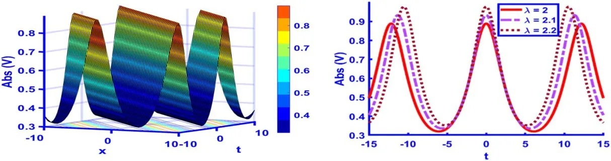
Figure 1.The 3D and 2D graphics for r ( t) =λt of the solution (24) with the parametric values h = 2,k = 1, α = 6, β = 2, γ=2 andλ = 2.

Figure 2 describes the periodic soliton nature represented by the solution (28).The suitable values of parameters withr(t)=λtare taken ash=0.5,k=0.2,α= 0.3,β= 0.4,γ= 0.6 andλ= 0.5 for 3D and 2D graphs.The twodimensional graph is portrayed atλ= 0.5,0.506,0.509 with different colors.The space-time range of 3D and 2D graphs is- 5 ≤x,t≤5.

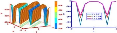
Figure 2.The 3D and 2D graphics for r(t) = λt of the solution(28)with the parametric values h= 0.5, k= 0.2,α = 0.3,β = 0.4,γ = 0.6 andλ = 0.5.

Also,the 3D graph in figure 3 reflects the bright solitonic nature forr(t) =sinh (λt)of the solution (28) with the appropriate parametric valuesh=0.7,k= -1,α= -1,β= 2,γ= 3 andλ= 0.2.The bright solitons are worthwhile to understand the behavior of charged carriers in quantum plasmas.The space-time range of 3D and 2D graphics is- 5 ≤x,t≤5.The two-dimensional plot is drawn atλ= 0.2,0.21,0.22 which are identified by diverse colors.

Figure 3.The 3D and 2D graphics for r ( t) =sinh ( λt)of the solution(28)with parametric values h =0.7, k= -1,α = -1,β = 2,γ = 3 andλ = 0.2.

On the contrary, the solution (29) for the parametric valuesh=4,k=4,α= 3,β= -0.1,γ= 0.3 andλ= 4 represents pulse like singular periodic soliton, presented in figure 4 forr(t)=λt.The singular solitons are traveling wave solutions having discontinuities.The time-space range for 3D graph is- 5 ≤x,t≤5,for 2D graph the time range is- 10 ≤t≤10 atλ= 4,5, 6.

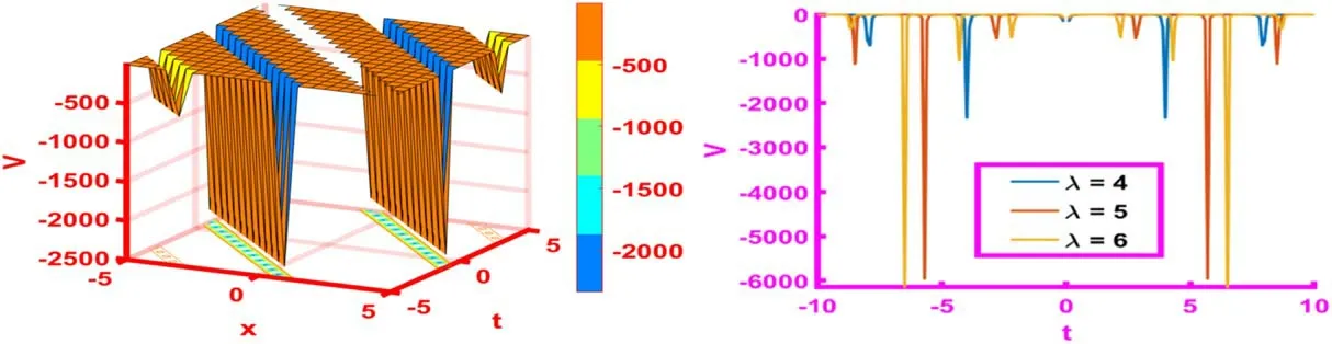
Figure 4.The 3D and 2D graphics for r ( t) =λt of the solution (29) with particular values h =4, k =4, α = 3, β = -0.1, γ = 0.3 andλ = 4.

Furthermore, the solution shapes in figure 5 show the compacton drawn from the solution (30) forr(t)=λt with the particular valuesh=2.8,k=3,α= 3,β= 2,γ= 1.9 andλ= 2.Compactons are a sort of soliton with a dense support that can be used to describe ion-acoustic waves,electrostatics wave, quantum acoustic waves in plasma physics.The space-time range for 3D graph is- 5 ≤x,t≤5.The two-dimensional plot is shown atλ= 2,2.1,2.2 in different colors with the time range- 10 ≤t≤10.

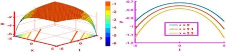
Figure 5.The 3D and 2D graphics for r ( t) =λt of the solution (30) with the particular values h =2.8, k =3, α = 3, β = 2, γ = 1.9 andλ = 2.

Figure 6 indicates the periodic soliton forr(t)=λt sketched from the solution (34) with the particular valuesh=0.7,k=1,α= 0.4,β= 0.4,γ= 0.6 andλ= -1.The time-space range of 3D graph for real and imaginary parts of the solution (34) is- 10 ≤x,t≤10.

Figure 6.The 3D graphics for r ( t) =λt of the solution (34) with the particular values h= 0.7, k= 1, α = 0.4, β = 0.4, γ = 0.6 andλ = -1.

Figure 7, describes the bell-shape soliton portrayed from the solution (38) forr(t)=λt with the parametric valuesh=0.7,k=1,α= 0.4,β= 0.4,γ= 0.6 andλ= 1.5.Bell-shaped solitons,which have infinite wings on both sides,are another sort of solitary wave solution useful signal management.The time-space range for 3D and 2D graph is- 5 ≤x,t≤5.The two-dimensional plot is portrayed atλ= 1.5,2,2.5.

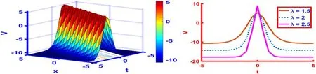
Figure 7.The 3D and 2D graphics for r ( t) =λt of the solution (38) with the particular values h= 0.7, k= 1,α = 0.4,β = 0.4,γ = 0.6 andλ = 1.5.

The solution (40) exhibits the parabolic soliton for the values ofh=9,k= -0.8,α= 2,β= 4,γ= 6 andλ= -0.1 withr(t)=λt sketched in figure 8.The space-time range of 3D and 2D graph is- 5 ≤x,t≤5.The twodimensional plot is depicted atλ= -0.1.

Figure 8.The 3D and 2D graphics for r ( t) =λt of the particular solution(40)with the parametric values h= 9, k= -0.8,α = 2,β = 4,γ = 6 andλ = -0.1.

The 3D graph in figure 9 shows the soliton nature fors(t) =sin (λt)of the particular solution (63) with the suitable parametric valuesl= -0.1,m=0.3,n=1,δ= 0.8,γ= 0.6,β= 0.9,α= 0.4 andλ= 0.2.The space-time range of 3D graph for real and imaginary parts of the solution(63) is- 10 ≤x,t≤10.

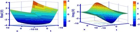
Figure 9.The 3D graphics for s ( t) =sin ( λt) of the solution(63)with the parametric values l= -0.1, m =0.3, n =1,δ = 0.8,γ = 0.6,β = 0.9,α = 0.4 andλ = 0.2.

On the other hand, figure 10 reflects the periodic soliton nature fors(t) =sin (λt) of the particular solution (66) with the particular valuesl=0.6,m=0.8,n=1,α= 2,β= 4,γ= 2,δ= 1 andλ= 1.The space-time range of 3D and 2D graph is- 8 ≤x,t≤8.Also, the 2D graph is depicted atλ= 1,1.2,1.4 which are specified by different colors.

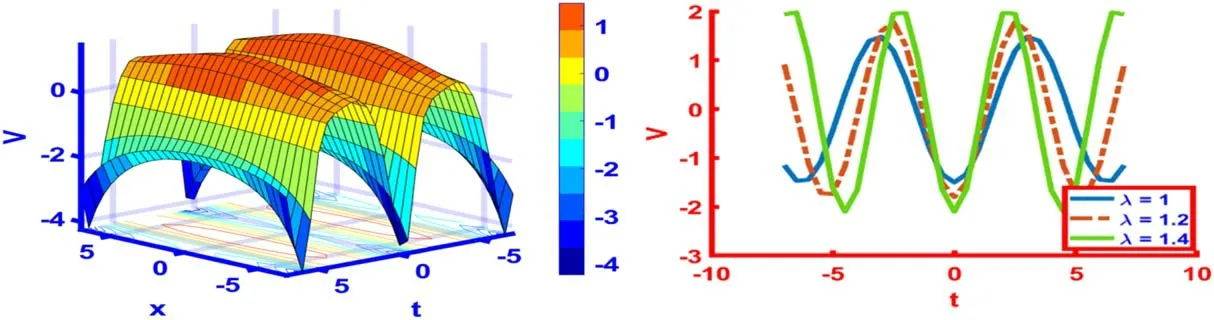
Figure 10.The 3D and 2D graphics for s ( t) =sin ( λt)of the general solution (66) with the parametric values l =0.6, m =0.8, n =1,α = 2, β = 4, γ = 2,δ = 1 and λ = 1.

Furthermore, the solution shapes in figure 11 is the bright-like soliton profile is interpreted from the solution(66)fors(t) =eλtwith the suitable parametric valuesl=5,m=0.5,n=2,α= 3,β= 1,γ= 2,δ= 2 and,λ= -0.4.This solution is descend from left to right asymptotic state.The space-time range for 3D and 2D graph is- 5 ≤x,t≤5.Also, the two-dimensional plot is illustrated atλ= -0.4,-0.5,-0.6.

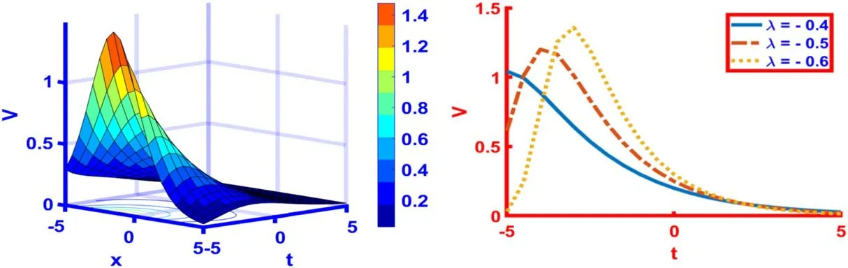
Figure 11.The 3D and 2D graphics for s ( t) = eλ t of the solution (66) with the particular values l =5, m =0.5, n =2,α = 3, β = 1,γ = 2,δ = 2 andλ = -0.4.

Figure 12 is the singular soliton characterized by the solution (67).The appropriate values of parameters withs(t) =sin (λt)are taken asl=1,m=0.2,n=0.9,δ= 1,γ= 1.5,β= 2.5,α= 1.5 andλ= 0.1 for 3D and 2D graphs.The two-dimensional graph is portrayed atλ= 0.1,0.2,0.3 with different colors.The space-time range of 3D and 2D graphs is- 5 ≤x,t≤5.

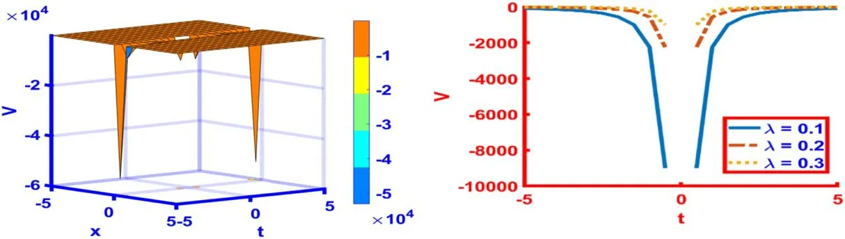
Figure 12.The 3D and 2D graphics for s ( t) =sin ( λt) of the particular solution (67) with the particular values l =1, m =0.2, n =0.9,δ = 1, γ = 1.5, β = 2.5, α = 1.5 andλ = 0.1.

Figure 13 represents the soliton like solution fors(t) =tanh (λt)of the solution (68) with suitable parametric valuesl=5,m=5,n=2,δ= 1,γ= 2,β= 1,α= 3 andλ= 0.4.The space-time range for 3D and 2D graphs is- 5 ≤x,t≤5.The two-dimensional plot is drawn atλ= 0.4,0.5,0.6 which are specified by different colors.

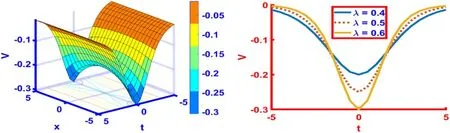
Figure 13.The 3D and 2D graphics for s ( t) =tanh ( λt) of the solution(68)with the particular values l =5, m =5, n =2,δ = 1,γ = 2,β = 1,α = 3 andλ = 0.4.

Figure 14, is periodic soliton depicted from the solution(75) fors(t) =cos (λt) with the suitable parametric valuesl=4,m=7,n=2.5,α= 3.5,β= 2.5,γ= 3.5,δ= 8 andλ= 0.6.The space-time range for 3D and 2D graph is- 5 ≤x,t≤5.The two-dimensional plot is shown atλ= 0.6,0.7,0.8 with different colors.

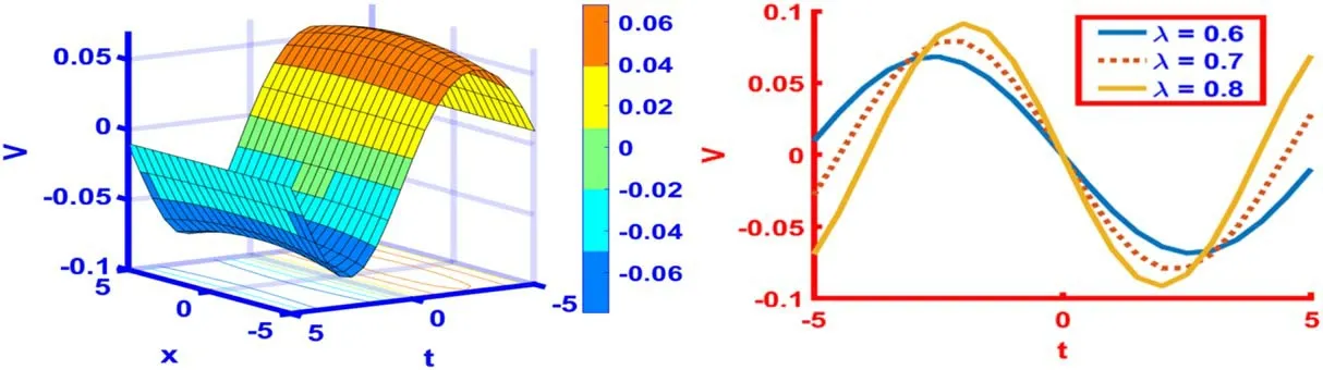
Figure 14.The 3D and 2D graphics for s ( t) =cos ( λt) of the particular solution (75) with the particular values l =4, m =7, n =2.5,α = 3.5, β = 2.5, γ = 3.5,δ = 8 andλ = 0.6.

Figure 15 signifies the singular soliton fors(t)=λt constructed from the solution (76) with the particular valuesl=1,m=7,n=5,α= 3,β= 0.5,γ= 1.5,δ= 1 andλ= 1.The time- space range of 3D and 2D graph is- 5 ≤x,t≤5.Also, the two-dimensional plot is depicted atλ= 1,2,3 which is shown in different colors.

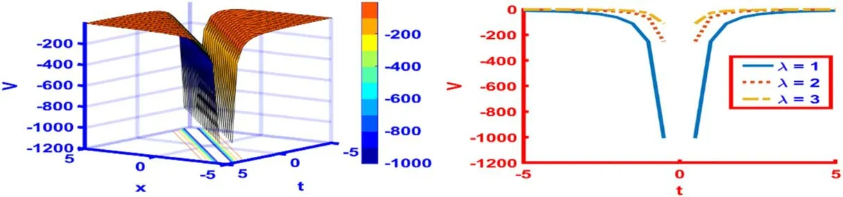
Figure 15.The 3D and 2D graphics for s ( t) =λt of the particular solution (76) with the particular values l= 1, m= 7, n= 5, α = 3,β = 0.5, γ = 1.5,δ = 1 andλ = 1.

The solution shape in figure 16 shows the plane soliton which is drawn from the solution (77) fors(t) =cos (λt)with the parametric valuesl= -0.9,m=7,n=2.5,α= 3.5,β= 2.5,γ= 3.5,δ= 8 andλ= 0.1.The space time range for 3D and 2D graph is- 5 ≤x,t≤5.Also, the two-dimensional plot is drawn at λ = 0.1,0.2,0.3 which are identified by three different colors.

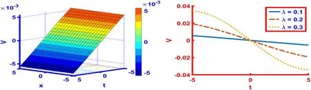
Figure 16.The 3D and 2 graphics for s ( t) =cos ( λt) of the solution (77) with the parametric values l= -0.9, m =7, n =2.5,α = 3.5,β = 2.5, γ = 3.5,δ = 8 andλ = 0.1.

For simplicity, some graphical representations of the achieved solutions are not reported here.Figures 1–16 indicate the periodic, bright, singular periodic, bell-shaped,compacton, parabolic, plane-shaped solitons etc describe the physical behavior of instances modulated by extended QZK equation and (3 + 1)-dimensional ZK equation.

5.Conclusion

In this study,we have effectively contrived the enhanced MSE technique to search for standard, definitive, and large-scale soliton solutions of the new extended QZK and (3 + 1)-dimensional ZK equations.The solutions are revealed in rational function, trigonometric function, hyperbolic function,exponential function and their integration.Bright solitons,periodic solitons, compacton, bell-shaped, parabolic, singular periodic solitons,plane shaped solitons,and some distinct and general solitons have been established.The soliton solutions that are similar to the preceding solutions validate this study,and the generic soliton solutions will enrich the literature and be valuable in future research.Two and three-dimensional graphs of these solutions are portrayed to help understand physical phenomena, namely ion-acoustic waves, dense quantum plasma, electron thermal energies, ion plasmas,quantum acoustic waves, quantum Langmuir waves, etc.This study confirms that the enhanced MSE technique is an effective and useful mathematical tool and is applicable to other NLEEs in physics, engineering and mathematical physics.

Acknowledgments

The authors would like to express their gratitude to the anonymous referees for their insightful remarks and ideas to improve the quality of the article.

ORCID iDs