LIMIT CYCLE BIFURCATIONS OF A PLANAR NEAR-INTEGRABLE SYSTEM WITH TWO SMALL PARAMETERS∗

(梁峰)

The Institute of Mathematics,Anhui Normal University,Wuhu 241000,China E-mail:liangfeng741018@126.com

Maoan HAN (韩茂安)†

Department of Mathematics,Zhejiang Normal University,Jinhua 321004,China Department of Mathematics,Shanghai Normal University,Shanghai 200234,China E-mail:mahan@shnu.edu.cn

Chaoyuan JIANG (江潮源)

The Institute of Mathematics,Anhui Normal University,Wuhu 241000,China E-mail:jcy7368591@126.com

Abstract In this paper we consider a class of polynomial planar system with two small parameters,ε and λ,satisfying 0< ε ≪ λ ≪ 1.The corresponding first order Melnikov function M1with respect to ε depends on λ so that it has an expansion of the form M1(h,λ)=.Assume that M1k′(h)is the first non-zero coefficient in the expansion.Then by estimating the number of zeros of M1k′(h),we give a lower bound of the maximal number of limit cycles emerging from the period annulus of the unperturbed system for 0<ε≪λ≪1,when k′=0 or 1.In addition,for each k∈ N,an upper bound of the maximal number of zeros of M1k(h),taking into account their multiplicities,is presented.

Key words Limit cycle;Melnikov function;integrable system

1 Introduction and Main Results

Consider the planar near-integrable system

where

ε>

0 is small,

p

(

x,y

)and

q

(

x,y

)are arbitrarypolynomials with degree

n

and independent of

ε,F

(

x,y

)is a particular polynomial with

F

(0

,

0)/=0

,

and the dot denotes a derivative with respect to the variable

t

.The unperturbed system of(1.1)has a period annulus around the origin.

Motivated by the works mentioned above,especially the method used in[14],in this paper we extend the bifurcation method with two small parameters of near-Hamiltonian systems[8]to consider limit cycle bifurcations of the near-integrable system

where 0

<ε

≪

λ

≪1 and

When

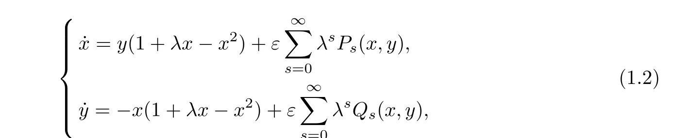
ε

=0,system(1.2)has a center at the origin and two parallel lines of singular points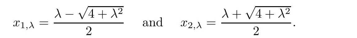

Note that 0

<

−

x

<x

for

λ>

0 small.Then,on the region|

x

|

<

|

x

|

,

system(1.2)is equivalent to the near-Hamiltonian system

whose unperturbed system has a family of periodic orbits given by

which forms a period annulus of systems(1.2)|and(1.4)|surrounding the origin,denoted by A.When

λ

=0

,L

(

h,λ

)reduces to

Corresponding to the family of periodic orbits,system(1.4)has the following first order Melnikov function in

ε

:

Where,by Lemma 2.1 in the next section,

Theorem 1.1

Consider system(1

.

2)with

n

∈Zand 0

<ε

≪

λ

≪1

.

Then,for

k

∈N,

2 Preliminary Lemmas

In this section we provide some preliminary lemmas in order to prove Theorem 1.1.

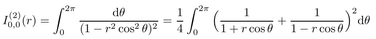
Lemma 2.1

For

k

∈N,the integral formula of

M

(

h

)in(1

.

8)holds.

Proof

Let

x

∈(−1

,

1)

.

Then,the perturbed terms of system(1

.

4)have the following expansions for 0

<λ

≪1: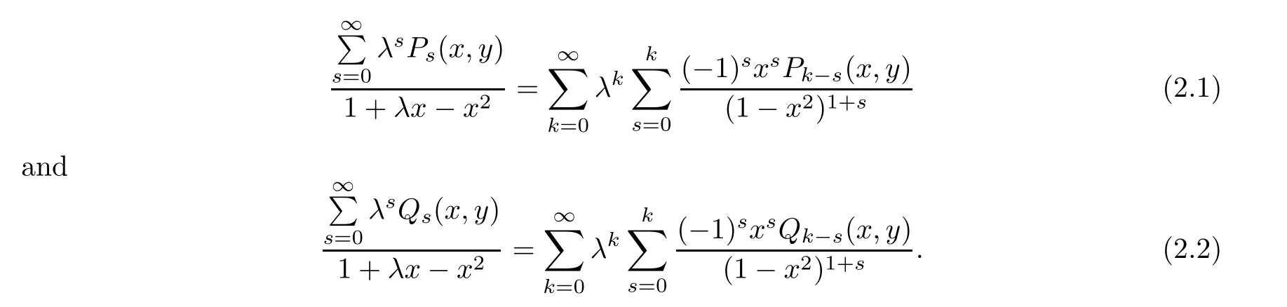

Inserting(2.1)and(2.2)into(1.6)yields

On the other hand,by(1.5),the first equality in(2.4)and the derivative formula in Lemma 2.1[8],we have

that is,

M

(

h,λ

)is independent of

λ.

Hence,(1.7),(2.3)and(2.4)together give

Lemma 2.2

Denote

Proof

The proofs of statements(i)and(ii)are straightforward.(iii)From(2.5),we have,for

i

∈N and

m

∈Z,

Thus,the statement(iii)holds.

(iv)Making a change

t

=

θ

−

π

,we get,from(2.5),that for

r

∈(0

,

1),

Then,by the integral formula

the first formula of(iv)is valid.

For the second formula of(iv),

which,together with the integral formula

and the first formula of(iv),yields

In view of(iii)and the first two formulae of(iv),it is clear that the third one of(iv)holds.

(v)Since,by(2.5),

Lemma 2.3

For

m

∈Z,

which is a polynomial in

r

of degree−

m

,and

ϕ

(

r

)denotes a polynomial in

r

with degree

m

−1 and

ϕ

(

r

)=2

π,ϕ

(

r

)=

π

(2−

r

)

.

Proof

We only give the proof of the case

m>

0 by mathematical induction.The proof for other two cases is clear.First,when

m

=1

,

2,the equality(2

.

6)holds,by the first two formulas of(iv)in Lemma 2.2,where

ϕ

(

r

)=2

π,ϕ

(

r

)=

π

(2−

r

)

.

Suppose that(2

.

6)works for

m

=3

,

4

,...,i.

Then,for

m

=

i

+1,we have,by the statement(v)of Lemma 2.2,that

is a polynomial in

r

of degree

i.

Therefore,(2

.

6)is obtained for all

m

≥1

.

Lemma 2.5

For

k

=1 or 3,

m,n

∈Zand

r

∈(0

,

1)

,

the following

m

+

n

+1 functions are linearly independent:

respectively.Obviously,for

k

=1 or 3,the functions in the above are linearly independent in the interval(0,1).Thus,the conclusion of the lemma follows.

3 Proof of Theorem 1.1

3.1 Proof of Theorem 1.1(i)

Set,for

n

≥1 and

r

∈(0

,

1),

Then,for

k

≥1,

Applying the statements(i),(ii)and(iii)of Lemma 2.2 in turn,we obtain that,for

k

≥1,

Then,by using very similar methods as to those in(3.7)–(3.8),we further have,by(3.11)and Lemma 2.3,that

By Lemmas 2.2 and 2.3,we note that in(3.15),

3.2 Proof of Theorem 1.1(ii)

Since,for

s

≥1 and

r

∈(0

,

1),

it follows that for

s

≥1,

Using(3.23),we have in(3.20)that

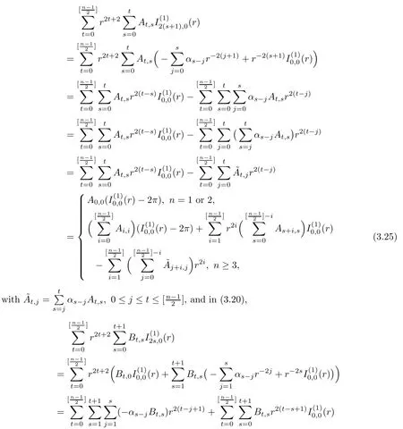
and when

n

≥2,

which,together with Lemmas 2.4 and 2.5,leads to

H

(1)≥2

.

For

n

=2,we have,similarly,that

and by Lemmas 2.4 and 2.5,

H

(2)≥2

.

When

n

≥3 is odd,substituting(3.33)and(3.41)into(3.30)shows that

where for

n

≥3 odd,we get

Recall that if for

n

≥3

,

can be chosen arbitrarily,then so can the coefficients

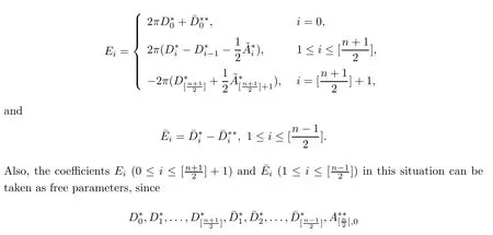
can be chosen arbitrarily and

Based on the discussions of the case

k

=1

,

we conclude that the statement of Theorem 1.1(ii)holds in this case.