Modeling hydrogen exchange of proteins by a multiscale method*

Wentao Zhu(祝文涛), Wenfei Li(李文飞), and Wei Wang(王炜)

School of Physics,National Laboratory of Solid State Microstructure,and Collaborative Innovation Center of Advanced Microstructures,Nanjing University,Nanjing 210093,China

Keywords: coarse-grained model, hydrogen exchange, multiscale method, proteins, integrative molecular

1. Introduction

Molecular dynamics(MD)simulation method is becoming an indispensable technique in the studies of biomolecular structures and dynamics due to its unprecedented spatial and temporal resolutions.[1-4]However, due to the sampling difficulties,conventional MD simulation at all-atom level can hardly access the timescales involved in most molecular motions of biological relevance. To overcome such efficiencybottleneck, many kinds of coarse-grained (CG) models have been developed and used in the simulations of biomolecules and prediction of functional sites of proteins.[5-11]In CG models,a group of atoms are represented by a single bead,so that the degrees of freedom can be largely reduced, which contributes to the increased simulation efficiency.[12]The main challenge of such CG models is that it is not straightforward to extract the CG force fields with high accuracy,which leads to the so called accuracy-bottleneck. Therefore, improving the accuracy of the CG models in biomolecular simulations attracts much effort in the fields of physics, chemistry, and biology.[6,7,11-15]Such efforts typically follow two lines: i) multiscale molecular simulations, in which information from all-atom simulations was used to improve the accessible accuracy of the CG models;[16-20]ii) integrative molecular simulations, in which restraints from available experimental data were used to improve the accuracy of the CG models.[21,22]With these improvements, CG simulations have shown great success in the studies of structure and functional motions for a wide range of biological systems,including molecular motors,[23]molecular chaperonin,[24]enzymes,[25,26]transcription machines,[27]nucleosomes,[28,29]and even chromosome.[30,31]

In literatures, many different kinds of experimental data have been used to restrain the MD simulations.Typical examples include the small-angle x-ray scattering(SAXS[32]), double electron-electron resonance (DEER[33]),F¨orster resonance energy transfer (FRET[34]), hydrogen exchange(HX[35])data,and so on. Hydrogen exchange(or hydrogen/deuterium exchange) is a powerful method in investigating the structural dynamics of proteins.[35-38]In HX experiments, the hydrogen atoms of proteins, particularly the protons in the backbone amide group, can exchange with the deuterium in D2O solvent, and the hydrogen exchange rate of a residue largely depends on its exposure extent to the solvent, which therefore can be used to characterize the structural dynamics of proteins in solution. Compared to the SAXS, DEER, and FRET techniques, the HX data can provide structural dynamics information at residue-level resolution. However, describing the HX data by MD simulations requires an all-atom level model, and previous studies have successfully used the HX data to restrain the all-atom MD simulations.[39,40]In order to use HX data to restrain the CG MD simulations,we need to develop a corresponding method to describe the HX data on the bases of the CG model.

In this work, we investigate the possibility to use the CG MD simulations to describe the HX data. For the CG simulations, we used an atomic-interaction based CG model(AICG2+),[41]in which the parameters were optimized based on all-atom MD simulations utilizing a multiscale strategy.Then by mapping the sampled CG structures back to the allatom structures,we calculated the HX protection factors. The results showed that such a combination of the CG simulations and structure mapping strategy can describe the experimental HX data reasonably well, which therefore builds up a bridge between the experimental HX data and the CG model. Particularly,we showed that the CG model can be further improved by integrating the available HX data via an iterative optimization process. All these results suggest that combining the CG model and HX data is a feasible strategy to achieve high accuracy and high efficiency MD simulations, which can help to extend the application cope of molecular simulations in the studies of biomolecular systems.

2. Method

2.1. Hydrogen exchange rates and local conformational equilibrium

According to previous HX model, hydrogen exchange occurs only when the amide hydrogen in a given residue of protein is exposed to the D2O, which requires the opening of the local conformation. The scheme can be described as following:[35-37,42]

Herekoprepresents the transition rate of the local conformation from the closed state(NHclosed)to the open state(NHopen),andkclis the rate of the reversal process.kchis the intrinsic exchange rate when the residue is fully exposed to D2O.The hydrogen exchange ratekexis then given by[37,42]

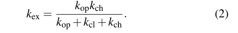
Under the EX2 limit(kch≪kcl)and the native-like conditions(kop≪kcl), the hydrogen exchange rate can be further written askex=KockchwithKoc=kop/kclbeing the equilibrium constant between open and closed states.[37,42]In HX experiments, the results were often given by the protection factor(P f),which is defined byPf=kch/kex,and it is related to the conformational equilibrium by

Therefore, the protection factorPfcan be directly derived from the equilibrated conformational distribution based on MD simulations.

2.2. Coarse-grained MD simulations

The MD simulations were performed by the atomicinteraction based CG model (AICG2+) developed in previous work.[41]In this model, each residue was represented by one spherical bead located at theCαposition. The AICG2+ energy function was constructed based on the perfect funnel approximation,[5]with the parameters being optimized based on all-atom MD simulations using a multiscale method.[41,43]The simulations were conducted by using the software CafeMol[10]with the temperature being controlled by the Langevin dynamics. The time step of the MD simulation was set as 0.1τ,withτbeing the CafeMol time unit. For each protein, we firstly conducted MD simulations at seven temperatures with the length of 5×108MD steps. Then the free energy landscape profiles at different temperatures were constructed by using the weighted histogram analysis method(WHAM[44]),from which we can determine the folding temperatureTf. Figure 1(b)shows the free energy profiles of the protein CI2 atT=1.0Tfand 0.92Tfprojected onto the reaction coordinateQ, which is defined as the fraction of formed native contacts at a given structure. AtT=1.0Tf, the free energy difference between the folded and unfolded states is zero according to the definition of the folding temperature. AtT=0.92Tf,the free energy difference is～11.5kBT,which is close to the experimental value measured at native condition for the protein CI2.[42,45]All the conformations sampled in the above simulations at different temperatures were reweighted to the target temperatureT=0.92Tfusing WHAM to model the protein dynamics at the native-like condition. We repeated the similar simulations for six different proteins, including CI2,Ubiquitin,SN,S6,HEWL,and IκBα,for which the HX data are available.[42,45-56]

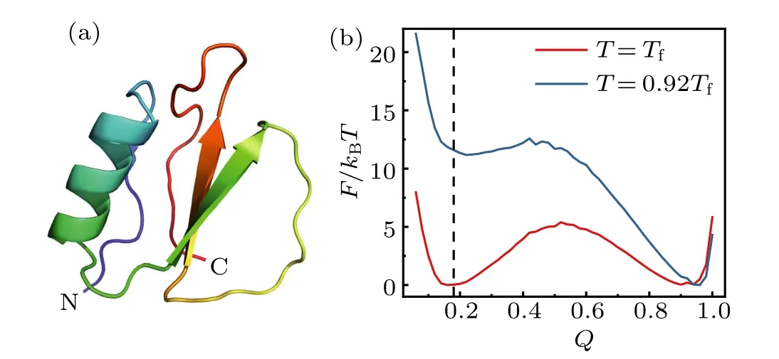
Fig. 1. (a) Cartoon representation of the three-dimensional structure of the protein CI2 (pdb code: 2CI2[57]). (b) Free energy profile of CI2 along the reaction coordinate Q at the temperatures of T =Tf and T=0.92Tf.The reaction coordinate Q represents the fraction of formed native contacts at a given structure.The dashed line denotes the Q-score of the unfolded state.

2.3. Calculations of HX protection factors

The relation between the experimental data of HX protection factor and the local conformational equilibrium propertyKocgiven by Eq. (3) provides a way to derive the protection factor values from MD simulation data. However,for the CG simulations, the local conformations are often poorly defined as the backbone amide groups contributing to hydrogen exchange are lacking, which makes the calculation of the protection factor a difficulty task. In this work, we introduced the reversal structure mapping strategy to overcome such difficulty. Firstly,we reconstructed the positions for all the backbone atoms starting from theCαpositions by using the BBQ program, which is a backbone building method from quadrilaterals and has been widely tested for the native and nearnative protein structures.[58]Then, the sidechain atoms were further reconstructed by using the software SCWRL based on the rotamer library, leading to the all-atom conformations for all the sampled CG structures.[59]Figure 2 shows the illustrative schematic for the reversal structure mapping using the BBQ and SCWRL for the protein CI2. With the obtained allatom conformations, one can calculate the equilibrium constant of the local conformations for each residue and therefore the protection factor.

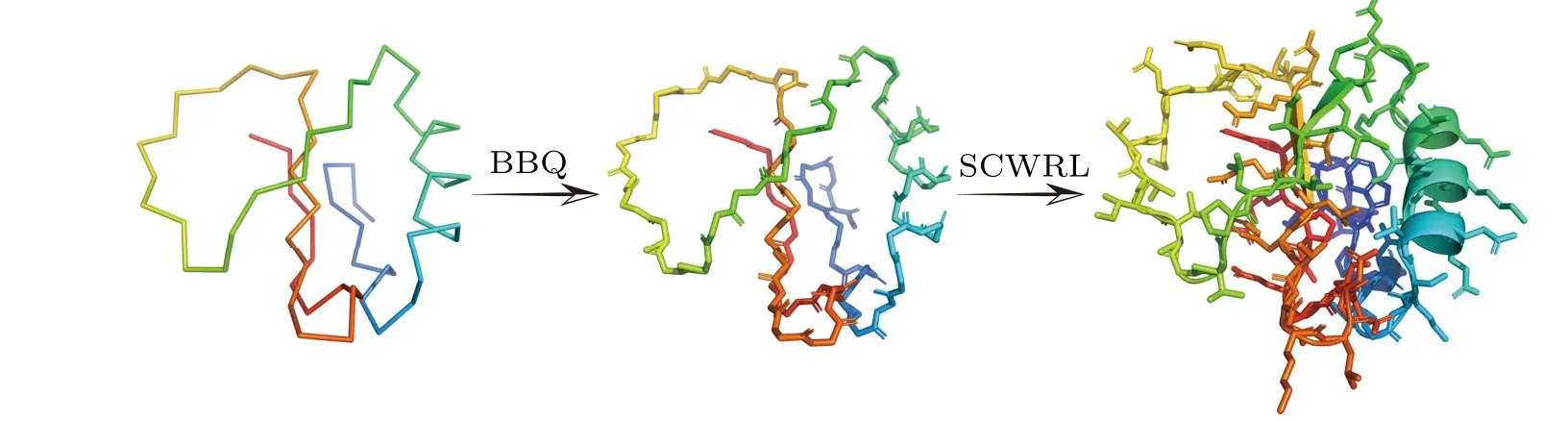
Fig.2. Illustrative scheme showing the all-atom structure reconstruction from Cα-based coarse-gained model of the protein CI2. At the first step,the positions of the backbone atoms were reconstructed by using the software BBQ.[58] Then the side-chain atoms were reconstructed by the software SCWRL.[59]

Several quantities can be used to characterize the exposure extent of the backbone amide groups from given allatom conformations,including the packing-density,hydrogenbond, solvent-accessible-surface-area, and so on.[37-39,60]In this work,we used the packing density and the number of hydrogen bonds.Here the packing densityNis given by the number of neighboring(within the distance of 6.5 ˚A)heavy atoms around the backbone nitrogen atoms for each residue. The hydrogen bonds involving the backbone amide groups were identified based on the distance cutoff of 3.5 ˚A and angle cutoff of 120°. The equilibrium constant can be approximately given by

Here〈···〉represents the weighted average among all the sampled conformations. IfKoc≈1, the residue is closer to the open state; otherwise, ifKoc≈0, the residue is closer to the closed state. Note that whenN ≫N0,the sigmoid function in Eq.(4)can be reduced to the exponential function,which was used in Refs. [38,39,60]. Based on Eqs. (3) and (4), the HX protection factor values could be extracted from the CG MD simulations. In Eq.(4),the parametersλ1,λ2,andN0were set as 10.0, 0.3, and 20, respectively. For the sake of simplicity,these values were used for all the residues without introducing amino acid type dependence in this work. The use of a common parameter set implies the assumption that the heavy atoms in different amino acids have similar contributions to the screening of the backbone amide group from solvent. In the subsequent section,we will show that even with such common parameter set for all the residues,the HX data can be reproduced reasonably well. It is possible that the performance of the above model can be further improved by introducing amino acid type dependence to these parameters.

3. Results

3.1. Comparison of HX data from MD simulations and experiments

In Ref. [42], the authors calculated the HX data for the proteins CI2,SN,and ubiquitin by using a more sophisticated protein model, in which more detailed structure information was included. Here we calculated the protection factors for the same set of proteins using the method described in Section 2. Figure 3 shows the results of the calculated protection factor(red lines in Figs.3(a),3(c),and 3(e)). For comparison,the results from experimental measurements are also shown(black dots and lines). The experimental HX data were taken from Ref.[42],which are the synthesis of the experimental results reported in Refs.[45-53]. One can see that for the above three proteins, the calculated results from the CG MD simulations with AICG2+model can reproduce the corresponding experimental data very nicely. Both the highly protected regions and the less protected protection regions can be well described,demonstrating the important role of native topology of proteins,as implied in the perfect funnel approximation[5-7,10]in defining the protein dynamics at native condition,which is consistent with previous discussions.[42]

To more quantitatively characterize the correlation between the simulation and experimental data, figure 3 also shows the correlation plots and the results of linear fitting(Figs. 3(b), 3(d), and 3(f)). The fitted Pearson’s correlation coefficientsRare 0.83, 0.73, and 0.68, respectively, for the three proteins. Such a correlation is comparable to the results reported in previous work with a more sophisticated model[42](Table 1),although the current model is much more simple and includes only theCαbeads. These results suggest that such a simple multiscale strategy,in which the CG simulations were combined with the structure reconstruction process to produce the all-atom structure ensemble, can be used to calculate the HX protection factors with reasonable accuracy. In the above calculations, we used the default parameter set given in Section 2. We also calculated the protection factors for the CI2 with theN0in Eq. (4) being set as 10, 15, 25, 30, 35, and 40. The resulted correlation coefficients with the experimental values are 0.82,0.83,0.83,0.83,0.82,and 0.80,respectively,which suggests that the results are insensitive to the parameterN0in the calculation of protection factors.

Fig.3. (a),(c),(e)HX protection factors from the CG MD simulations(red)and experimental data(black)for the residues of the proteins CI2(a),ubiquitin(c),and SN(e). (b),(d),(f)Correlation plots between the experimental protection factors and the calculated values with AICG2+force field for the proteins CI2 (b), ubiquitin (d), and SN (f). The red straight lines represent the results of linear fitting. The fitted Pearson’s correlation coefficients R were also shown in each panel.

Table 1. The fitted Pearson’s R between the protection factors from CG MD simulations with the AICG2+model and the experimental data for six proteins. The results from previous work[42] were also shown for comparison.

We also repeated the above calculations for another three proteins, including the S6, HEWL, and IκBα. The experimental data were taken from Refs. [54-56], respectively. As shown in Table 1, the calculated correlation coefficients are larger than 0.6 for S6 and HEWL, demonstrating reasonable correlation between the CG simulations and the experimental data for these proteins.In comparison,the obtained correlation coefficient for the IκBαis 0.55,which is significant but much smaller than the values of other proteins discussed above,suggesting the defects in the used CG model. In the next subsection, we will investigate whether it is possible to improve the description of the HX data by optimizing the force field parameters of the above CG model.

3.2. Restraining the CG simulations with HX data

The above results clearly demonstrated the correlation between the simulated HX data and the experimental HX data.However,as shown in Table 1,the correlation coefficients for different proteins can be very different. For the protein CI2,the correlation coefficient is 0.83,which is the highest among the studied proteins in this work. In comparison, the correlation coefficient for the IκBαis much lower(0.55),suggesting the defects of the used CG model in describing the HX data.Meanwhile,the observed correlations encouraged us to investigate whether we can use the HX data to restrain the CG MD simulation and obtain better description of the experimental data. To this end, we constructed an iterative scheme to optimize the parameters of the CG model with the input from experimental data. Specifically,we firstly run MD simulations based on the old CG force field and calculate the protection factor values as described above. Then,we update the parameterεiby using the following formula:

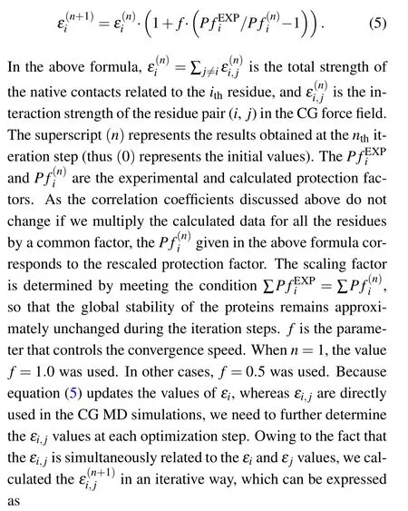
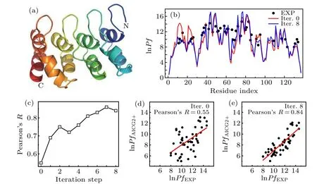
Fig. 4. (a) The cartoon representation of the native structure of IκBα (pdb code: 1NFI[61]). (b) Comparison between the experimental and calculated protection factors(rescaled)before iterative optimization(red)and after eight steps of iterative optimization(blue).(c)The Pearson’s correlation coefficient R as a function of iterative optimization steps. (d), (e) The linear correlation between the experimental and predicted protection factors (not rescaled) before iterative optimization (d) and after eight steps of iterative optimization (e). The red straight lines represent the linear fit. The obtained Pearson’s correlation coefficients R were also shown.

Fig. 5. (a) The differences between the interaction strengths εij of the native contacts before iterative optimization and after eight steps of iterative optimization. Red/blue color represents that the interaction strengths become stronger/weaker after optimization. The unit of the color scale is kcal/mol. (b)Same as(a)but with the differences of the εij averaged among all the contacting partners of a given residue. (c)Same as(a)but with the differences of the εij averaged among all the contacting partners of the residues with a given amino acid type.

Figure 4(c)shows the Pearson’s correlation coefficientRfor the protein IκBαas a function of the optimization step.One can see that the correlation coefficient increases gradually with the progression of optimization. Before optimization, the correlation coefficient is 0.55. After eight steps of iterative optimizations,the correlation coefficient increases to 0.84 and gets saturated. The final values of the calculated protection factors show great consistence with the experimental data (Figs. 4(b), 4(d), and 4(e)). Notably, the results around the residue 20 were largely improved due to the better description of the relative stabilities for the first and second helices.Figure 5 shows the differences between the non-bonded interaction strengthsεijbefore iterative optimization and after eight steps of iterative optimization.One can see that the interaction strengths involving the residues with index around 20 become weaker (Fig. 5(a), blue circle line), whereas those involving the residues with index around 70 become stronger(Fig.5(a),red circle line),which is consistent with the observed changes of the HX data in Fig.4. Similar results can be obtained from the differences of theεi javeraged among all the contacting partners of each given residue(Fig.5(b)). However,effect of optimization does not show obvious amino acid type dependence(Fig.5(c)).Such results demonstrate that with the above iterative optimization scheme, the information from HX data can be effectively integrated into the CG force field to improve the description of the protein structural dynamics by CG MD simulations.

4. Discussion and conclusion

The above results demonstrated that we can improve the CG force fields based on the HX data, although the CG MD simulations were related to the experimental data of the HX by an indirect manner involving an intermediate step of structure reconstruction. Possible reason is that with theCαpositions,the corresponding all-atom structure was relatively well defined as demonstrated in previous works,[58,59]especially for the structures at the native-like conditions discussed in this work. Apparently, the accuracy of such integrative molecular simulation scheme relies on the performance of the structure reconstruction algorithm. In recent years,developing new structure reconstruction algorithms becomes the focus of several research groups.[62-64]We believe that with the further improvements of accuracy and efficiency of the structure reconstruction algorithms,the description of the HX data by the CG MD simulations will become more plausible, which can then promote the developments and applications of the integrative molecular simulations with the combinations of the CG model and HX data. Such a combination has obvious advantages.Firstly, the HX data can provide residue-level structural dynamics information,which is superior to other low-resolution experimental data widely used in previous integrative molecular simulations. Secondly,the CG model often has the advantage of high sampling efficiency,but encounters accuracy bottleneck. Because imposing experimental restraints mainly improves the accuracy aspect(instead of the sampling efficiency)of the simulations,such combination can help to overcome the major bottleneck of the CG simulations.

In summary, we used a multiscale scheme to calculate the HX protection factors, in which the structure reconstruction algorithms were used to convert the sampled structures by CG MD simulations into all-atom detailed structures,from which we can calculate the HX protection factors. By using this method,the HX data can be described with reasonable accuracy by the CG MD simulations. In addition, we showed that the CG force field parameters can be further improved by iterative optimization based on the available experimental data of the HX experiments. Such a combination of the CG MD simulations and HX data can be applied to the studies of other protein dynamics of biological relevance.

Acknowledgment

We thank the insightful discussions with Shoji Takada.