Evaluating the eff ect ofinput variables on quantifying the spatial distribution of croaker Johnius belangerii in Haizhou Bay, China*

Yunlei ZHANG , Ying XUE ,3, Binduo XU ,3, Chongliang ZHANG ,3, Xiaoxiao ZAN

1 College of Fisheries, Ocean University of China, Qingdao 266003, China

2 Marine College, Shandong University, Weihai 264209, China

3 Field Observation and Research Station of Haizhou Bay Fishery Ecosystem, Ministry of Education, Qingdao 266003, China

Abstract A habitat model has been widely used to manage marine species and analyze relationship between species distribution and environmental factors. The predictive skill in habitat model depends on whether the models include appropriate explanatory variables. Due to limited habitat range, low density,and low detection rate, the number of zero catches could be very large even in favorable habitats. Excessive zeroes will increase the bias and uncertainty in estimation of habitat. Therefore, appropriate explanatory variables need to be chosen first to prevent underestimate or overestimate species abundance in habitat models. In addition, biotic variables such as prey data and spatial autocovariate (SAC) of target species are often ignored in species distribution models. Therefore, we evaluated the eff ects ofinput variables on the performance of generalized additive models (GAMs) under excessive zero catch (＞70%). Five types ofinput variables were selected, i.e., (1) abiotic variables, (2) abiotic and biotic variables, (3) abiotic variables and SAC, (4) abiotic, biotic variables and SAC, and (5) principal component analysis (PCA) based abiotic and biotic variables and SAC. Belanger’s croaker Johnius belangerii is one of the dominant demersal fish in Haizhou Bay, with a large number of zero catches, thus was used for the case study. Results show that the PCA-based GAM incorporated with abiotic and biotic variables and SAC was the most appropriate model to quantify the spatial distribution of the croaker. Biotic variables and SAC were important and should be incorporated as one of the drivers to predict species distribution. Our study suggests that the process ofinput variables is critical to habitat modelling, which could improve the performance of habitat models and enhance our understanding of the habitat suitability of target species.

Keyword: generalized additive model; principal component analysis; biotic variables; spatial autocovariate

1 INTRODUCTION

Identifying the habitat and spatial distribution of species is important for fishery management and marine biological conservation (Bailey and Thompson, 2009), especially for species that are susceptible to environmental variations (Sagarese et al., 2014; Peck et al., 2018). With fisheries management moving to ecosystem-based approaches(Pikitch et al., 2004; Dolan et al., 2016), spatial information for target species becomes even more important (Giannoulaki et al., 2013; Marzloff et al.,2016; Xue et al., 2018). Several data-driven multivariate statistical methods like multiple linear regression, generalized linear models (GLM),generalized additive model (GAM) and machine learning methods are usually used for analyzing the relationship between explanatory variables and habitats of species (Guisan et al., 2002; Ahmadi-Nedushan et al., 2006; Jordaan et al., 2010; Li et al.,2017; Liu et al., 2019). Among them, GAM can determine the complex nonlinear relationship between response variables and input variables (Kitchens and Rooker, 2014), thus providing a flexible and robust method for predicting the spatial distribution of species (Schmiing et al., 2013; Zerbini et al., 2016).

The limited habitat range, low density, and low detection rate might result in a large number of zero catches (Martin et al., 2005; Virgili et al., 2017) and positive skewed distribution of species abundance.Excessive zeroes will increase the bias and uncertainty in estimation of model parameters (Martin et al.,2005), which is a challenge for determining the existence of the specie (Lee et al., 2006; Virgili et al.,2017). In addition, ecological data are often overdispersed with the variance being greater than the mean. Therefore, appropriate process of explanatory variables before habitat modelling is necessary to avoid biased predictions (Lee et al., 2006).

The spatial distribution of species can be predicted in habitat models based on environmental variables(Guisan and Thuiller 2005; Gormley et al., 2011;Virgili et al., 2017). Abiotic variables, such as spatial variables and environmental variables, are often used as explanatory variables to predict the spatiotemporal distribution of species. However, biotic variables such as prey data are also one of the important factors driving the predator’s distribution and cannot be ignored in species distribution models (SDMs) (Bi et al., 2011; Murase et al., 2013; Arrizabalaga et al.,2015; Zerbini et al., 2016). Including prey data has been proved capable ofimproving the predictive skills of SDMs (Cormon et al., 2014; Vezza et al.,2015; Xue et al., 2018). However, prey data have rarely been considered due to the lack ofinformation of non-commercial prey species, which may lead to incomplete and biased predictions of predator’s distribution (Johnson et al., 2013). Understanding the relationship between species distribution and related abiotic and biotic variables can provide critical information to predict abundance and identify suitable habitats of marine organisms (Murase et al., 2013;Vezza et al., 2015).

Multicollinearity between variables needs to be assessed and addressed before habitat modeling (Xue et al., 2018). However, removing some variables by statistical methods such as residual regression,ordinary least squares, and ridge regression, may lead to important information missing. In this case, the principal component analysis (PCA) is preferred to reduce the dimension of variables with the principal components (PCs), which can eff ectively retain significant information and avoid collinearity(Ahmadi-Nedushan et al., 2006; Buisson et al., 2008).In addition, incorporating spatial autocovariate (SAC)of target species into habitat models can also improve the performance of SDMs, especially when significant SAC was detected in the residuals (Wu et al., 2009).

The aim of our study was to evaluate the eff ect ofinput variables on the performance of habitat models.Belanger’s croaker (Johnius belangerii) collected from the bottom trawl surveys in Haizhou Bay with a large number of zero catches was selected as target species. We evaluated the eff ects of diff erent types ofinput variables (i.e., abiotic variables, abiotic and biotic variables, abiotic variables and SAC, abiotic and biotic variables and SAC, and PCA-based variables) on the performance of GAM, and their ability to deal with the over-dispersed dataset were also evaluated. The process ofinput variables selection is critical in habitat modelling, and optimal combination ofinput variables is expected to improve the predictive performance of habitat models and deepen our understanding of species spatiotemporal distributions.

2 MATERIAL AND METHOD

2.1 Data collection

Belanger’s croakers (Johnius belangerii) were collected from bottom trawl surveys in Haizhou Bay and the adjacent areas on spring (May) in 2011 and 2013-2018 (Fig.1). The survey area spans 119°20′E-121°10′E, 34°20′N-35°40′N. Stratified random sampling was used for investigation (Xu et al., 2015).In accordance with the diff erences in geological,oceanographic and biological characteristics of the survey area, a certain number of stations were randomly selected in each stratification (Xu et al.,2015). Twenty-four stations were selected in 2011,and the sampling stations were optimized to 18 after 2013 (Xu et al., 2015; Zhang et al., 2020). The bottom trawl was towed at 2-3 knots for about 1 h, with a trawl mesh size of 17 mm and net of 12 m width(Zhang et al., 2020). Tows were only conducted during daytime (6:00-18:00). At each survey station,GPS was used to record the sampling location. At the same times, CTD system (XR-420) was used to measure environmental data including temperature,salinity, and depth. The distance between sampling station and the nearest coastline was determined geographically (Zhang et al., 2020). To account for spatial autocorrelation, we included a measure of thesurrounding mean abundance ofJ. belangeriiin the Voronoi diagram (Muramatsu et al., 2018) as a SAC(Fig.2). The survey data were standardized by 2 knots and 1 hour, and the catch number per unit area (inds./km2) was used as the abundance index (Liu et al.,2019; Zhang et al., 2020).

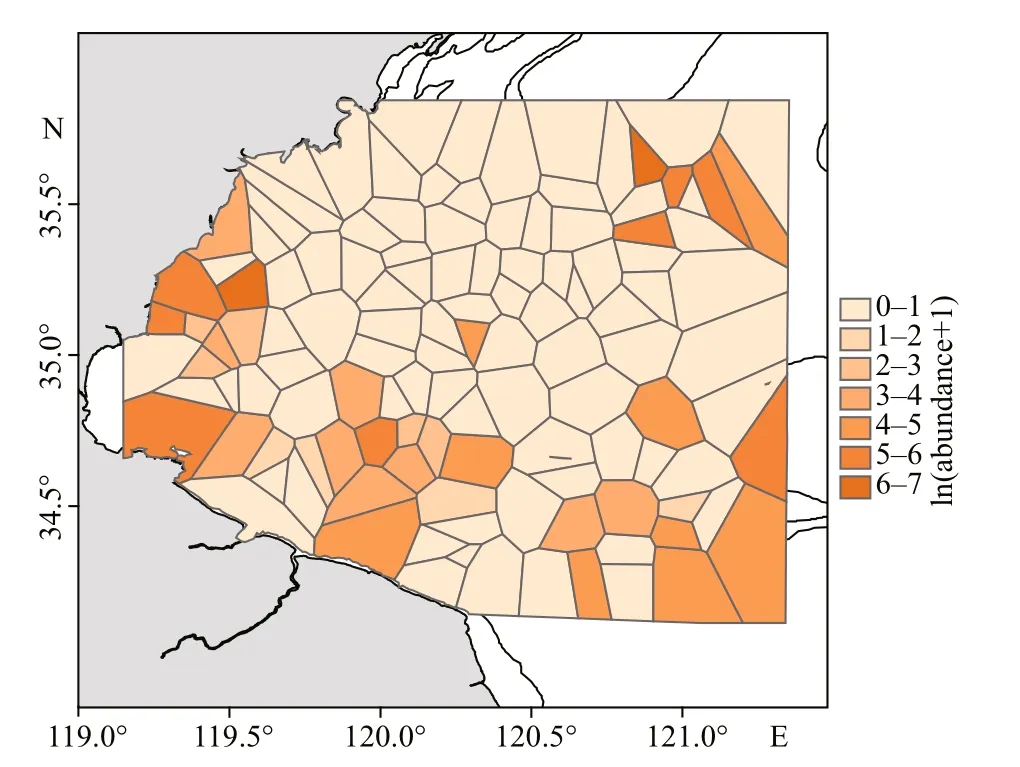
Fig.2 The Voronoi diagram of J. belangerii abundance in the study areas in the springs of 2011 and 2013-2018

2.2 Stomach contents analysis

The stomach contents ofJ. belangeriiwere analyzed based on 166 stomach samples. In laboratory,prey items were identified to the lowest possible taxonomic level and calculated weight for each content (Paquin et al., 2014). The index of relative importance (IRI) and the percentage of relative importance index (%IRI) were calculated to describe the relative contribution of prey species in the diet(Guedes et al., 2015).

where %Wis the percent of weight of prey species,%Nis percent of number, %Fis frequency of occurrence, andnis the total number of prey items.

2.3 Candidate explanatory variables

The abiotic explanatory variables included bottom temperature, bottom salinity, depth, distance off shore,and year. The dominant prey species ofJ. belangeriiwere chosen as biotic variables in the modeling. The prey species were synchronously collected in each survey station by bottom trawl surveys in Haizhou Bay. The mean abundance ofJ. belangeriiin the Voronoi diagram was chosen as SAC. In this study,five types ofinput variables were used for modeling,including (1) abiotic variables only, (2) abiotic and biotic variables, (3) SAC and abiotic variables, (4)SAC and abiotic and biotic variables, and (5) PCAbased SAC, abiotic, and biotic variables. Before modeling, highly correlated explanatory variables were excluded from model by variance inflation factors (VIF) to avoid collinearity (Li et al., 2017;Luan et al., 2018). Previous studies showed that the variable whose VIF is ＞2 indicates strong collinearity (Kabacoff , 2015; Zhang et al., 2020), thus it was dropped from the modeling. The VIF value was determined using the vif function in “car” package of R software (version: 3.4.2) (Zhang et al., 2020).

2.4 Generalized additive model (GAM)

GAM is the generalization oflinear regression model and additive in the predictor eff ects (Zhang et al., 2020). GAM is expressed as:

whereYis abundance of species,αis the intercept term,fi() is a smooth function of explanatory variables spline,xiare explanatory variables,nis the number of predictors, andεis the residual error term (Hastie and Tibshirani, 1986; Zhang et al., 2020).

For the PCA based GAM, we applied PCA to analyze the uncorrelated explanatory variables. The PCA informed GAM can be described as follows:

wherepciare principal components. In order to avoid overfitting, all the smoothers were constrained with 4 knots. The models were fitted withtwfunction(Tweedie distribution) usingmgcvpackage of R software (Wood, 2006). The principal components were chosen with eigenvalue more than 1 (Buisson et al., 2008; Liu et al., 2019).

The response variable was linked to the additive predictors using a log-link function. The significant variables were selected by stepwise procedure. It started with a null model and added one predictive variable to the present model at each step (Luan et al.,2018; Zhang et al., 2020). Akaike Information Criterion (AIC) (Akaike, 1998) was used for variable selection, in which GAM with the lowest AIC value was regarded as the best model (Luan et al., 2018;Zhang et al., 2020). We extracted the percentage of variance explained, and checked the distribution of residuals for all models. Important variables were selected step by step in procedure starting with an empty model and adding a predictor variable to the current model in each step.

2.5 Model evaluation

We evaluated the performance of diff erent GAMs in describing the spatial distribution ofJ. belangeriiin Haizhou Bay. The abundance was log-transformed(ln(x+1)) to reduce the influence of extreme values and meet the requirement of error distribution in GAMs (Zhang et al., 2018a). Cross-validation was applied to assess the performance of GAMs (Guisan and Zimmermann, 2000; Mouquet et al., 2015; Yu et al., 2018). About 70% of the data subset was randomly selected for model development, and the remaining 30% were used to evaluate the performance of the habitat models (Smith, 1994; Zuur et al., 2007; Zhang et al., 2020). For each GAM, cross-validations were run for 100 times and linear regression between the observed and predicted abundance ofJ. belangeriiwas analyzed at each run (Xue et al., 2018, Zhang et al., 2018a). The predicted abundance distributions were mapped using ordinary kriging in AcrGIS. The performance of each GAM was evaluated according to the regression coeffi cient of determination (R2), the root mean square error (RMSE), the intercept, and the slope between the predicted and observed abundance data (Brennan et al., 2019). The model with the maximumR2, the minimum RMSE was selected as the optimal model (Brennan et al., 2019).

3 RESULT

The abundance ofJ. belangeriiin the studied area ranged from 0 to 826.464 inds./km2, on average of 40.841±10.282 inds./km2. Inter-annual variation of the abundance was observed, from the highest(118.064±50.185 inds./km2) in 2016 to the lowest(4.354±3.500 inds./km2) in 2018.

14.Goody: A more exact translation of Perrault s French would be my dear lady. Goody is short for Goodwife or Goodwoman (usually used for the middle classes), a polite term of address such as Mrs. or Ms. is today, but slightly more familiar.Return to place in story.

3.1 Diet composition

Decapoda and amphipoda were main prey groups ofJ. belangerii, with %IRI being 45.248% and 50.403%, respectively, followed by polychaeta(2.323%), and euphausiacea (1.798%). There were 19 prey species in total, of whichLatreutesanoplonyx,Parapenaeopsistenella,Alpheusdistinguendus, andLatreutesplanirostrisdominated (Table 1). The total weight percentage in the diet was 55.336%. These four major prey species were selected as the biotic variables in habitat modeling.

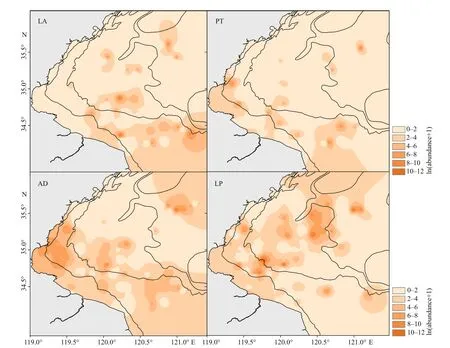
Fig.3 The spatial distribution of four major prey species of J. belangerii during spring in 2011 and 2013-2018 in Haizhou Bay

3.2 Spatial overlap between J. belangeriiand its major prey

Johnius belangeriimainly concentrated in the center and southern coastal waters of Haizhou Bay.Diff erence in spatial distribution of the four prey species was obvious (Fig.3).L.anoplonyxdistributed mainly in the southeastern and center area of Haizhou Bay.P.tenellaandA.distinguendusgathered in the central and southern coastal waters, which is similar to the distribution ofJ. belangerii. However,L.planirostrisamassed in the central and northern areas of Haizhou Bay, which was diff erent fromJ.belangeriiand other prey in the regard.

Johnius belangeriiwas found to mainly inhabit in the areas overlapped with its main prey species(Fig.4). In addition, there was a significant correlation(R2=0.527,P＜0.01) between abundance ofJ.belangeriiand its four major prey species. The fluctuation patterns in abundance betweenJ.belangeriiand the four prey species were similar from 2011 to 2018.

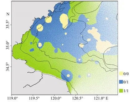
Fig.4 The spatial location relationship between J. belangerii and its four main prey species

3.3 Variables selection

Nine potential explanatory variables were selectedas candidate variables to explore the performance of GAMs (Table 2).

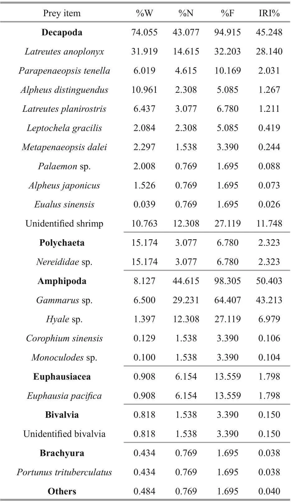
Table 1 Diet composition of J. belangerii in Haizhou Bay

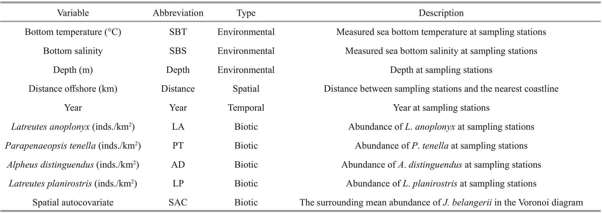
Table 2 Potential explanatory variables in GAMs for J. belangerii in Haizhou Bay

Overall, four GAMs with diff erent combination of candidate variables were built, including GAM1 with only abiotic variables, GAM2 with abiotic variables and SAC, GAM3 with abiotic and biotic variables,and GAM4 with all abiotic, biotic variables and SAC.The degree of multicollinearity was measured by VIF(Table 3). The VIF values of candidate variables were all less than 2 in the four groups. Therefore, all factors were kept for GAMs modeling.

The PCA revealed four optimal principal components (Fig.5) whose cumulative of variance was 0.72 (Table 4). The higher loading values in PC1 were contributed by abiotic variables with proportion of variance at 0.30, while those for biotic variables,year and biotic variables, and SAC variables were 0.16, 0.15, and 0.11, respectively (Table 4).

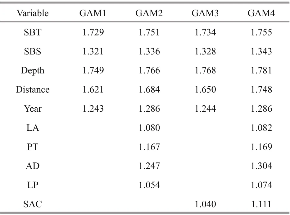
Table 3 Test of multicollinearity among abiotic, biotic variables and spatial autocovariate in four GAMs

3.4 Model fitting and evaluation

GAMs with diff erent input variables exhibited diff erent performance for model fitting. The explained deviances ranged from 19.40% for GAM1 with only abiotic variables to 55.60% for GAM5 with PCA based variables (Table 5). In addition, the highest determination coeffi cient (R2) was found in GAM5(0.497), while the lowestR2was in GAM1 (0.162).Overall, GAM5 with PCA based variables performed better than the other GAMs, which had the highest values ofR2and deviance explained.

The predicted abundance ofJ. belangeriiincorporating biotic variables and SAC into input variables had higher correlation with observed abundance, especially for GAM5 with PCA based variables (Fig.6). The correlation coeffi cients between predicted and observed abundance ofJ. belangeriiduring spring from 2011 to 2018 in Haizhou Bay ranged from 0.445 (GAM1) to 0.808 (GAM5) (Fig.7).

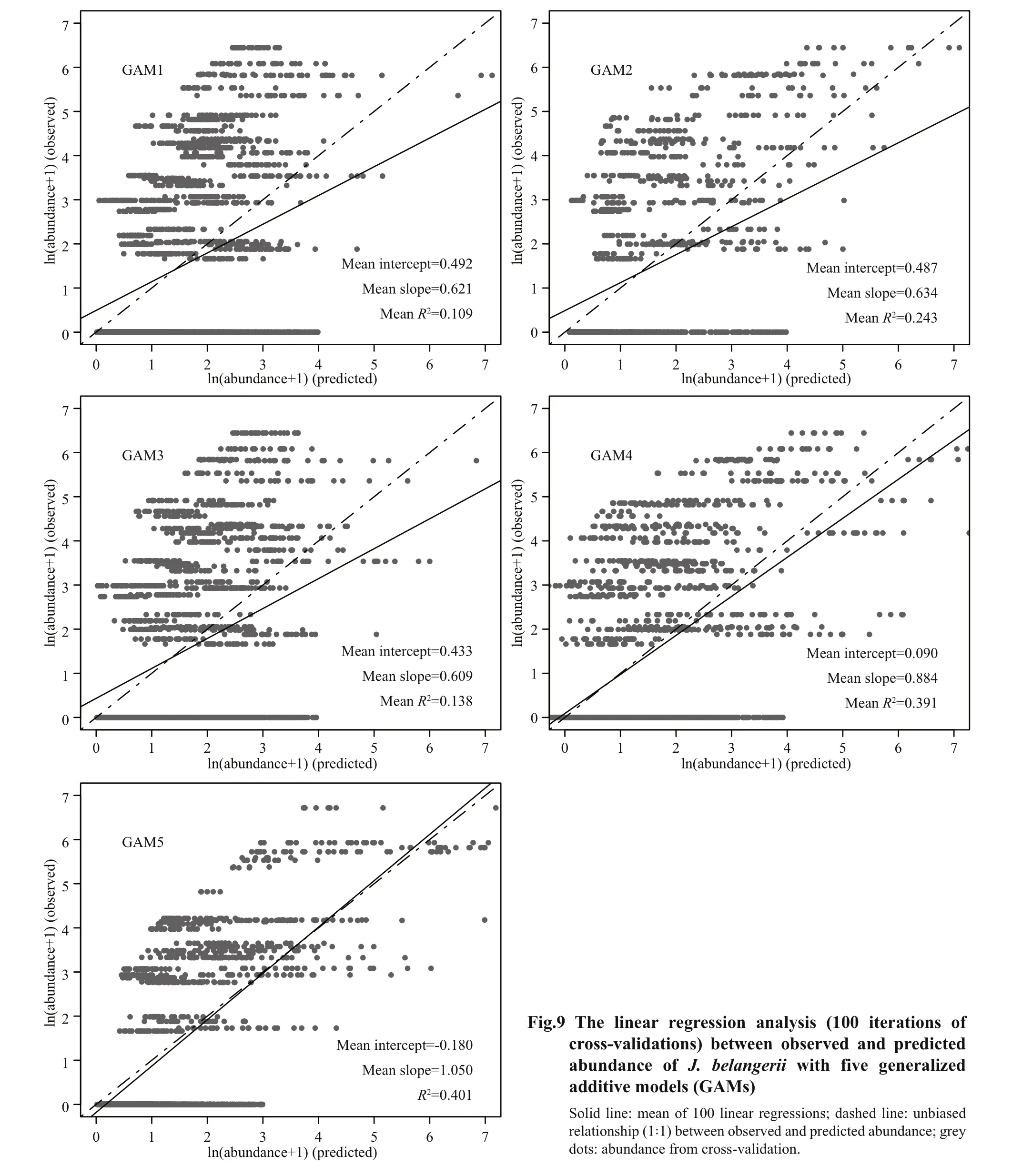
For cross-validation,R2of all GAMs ranged from0.01 to 0.68 and RMSE ranged from 1.06 to 3.69(Fig.8). Among the five GAMs, GAM5 showed the best performances than other models, with the highestR2and lowest RMSE. The overall predictive performance of the five GAMs was evaluated by linear regression analyses between observed and predicted abundance ofJ. belangerii. Results reveal that GAM5 performed better than the other four GAMs, with the highest slope andR2closest to 1. A tendency to underestimate the abundance ofJ.belangeriiwas observed in the other four GAMs(Fig.9), and the degree of underestimation increased with higher prevalence.

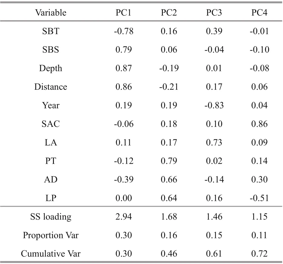
Table 4 Loadings of each variable in the first four principal components (PCs)

4 DISCUSSION

Habitat models can be used to identify key areas of protection to meet stakeholder’s expectations(Cañadas et al., 2005). However, it is diffi cult to find a balance between high explanatory power and the elimination of random noise in the model (Li et al.,2015). In addition, for response variable, neglecting the eff ect of over-dispersion may lead to the selection of models to be more complex than necessary(Richards, 2008), where the model is not generalized outside of the sample used for calibration (Virgili etal., 2017). Therefore, selecting appropriate model and input data are critical in the habitat modelling,especially for species that are barely detected, with their high-density regions being diffi cult to be identified.

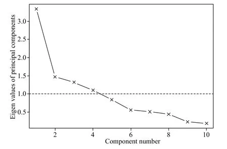
Fig.5 The principal components selected in habitat modeling

Table 5 Summary of the five GAMs for J. belangeriiin Haizhou Bay

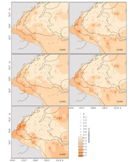
Fig.6 Overlaid maps of observed (black circles) and predicted (color contours) abundance of J. belangeriibased on five GAMs during spring in Haizhou Bay

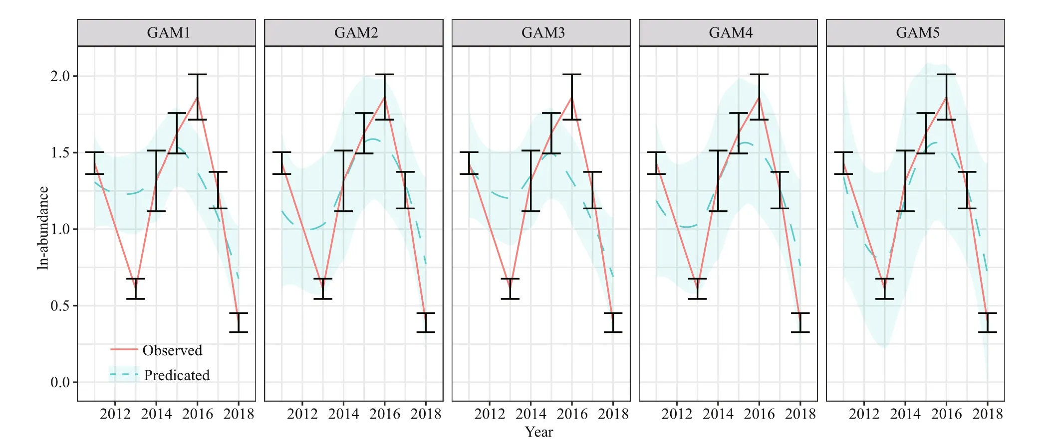
Fig.7 Predicated and observed mean abundance of J. belangerii during spring from 2011 to 2018 in Haizhou Bay based on five GAMs

Johnius belangeriiis one of the dominant fish species in the study area (Zhang et al., 2018b). It is a demersal fish and likes to inhabit shallow waters with warm temperate. Spring is the main spawning season and Haizhou Bay serves as the main spawning ground forJ. belangerii. Based on the three environmental variables, i.e. SBT, SBS, and depth, Zhang et al.(2018b) studied the habitat suitability ofJ. belangeriiduring spring in Haizhou Bay. The study found that depth and SBT were the main factors aff ecting the distribution ofJ. belangerii. The optimal habitat ofJ.belangeriivaried with life history stage. The distribution of suitable habitat was closely related to external environmental factors.J. belangeriihas a patched spatial distribution pattern. In trawl surveys,more than 70% of sampling stations have the abundance value of zero, which has an obvious overdispersed dataset. Compared with other generalist feeders,J. belangeriihas more specified feeding habits (Xiao et al., 2019), with a few major prey species that may have significant impacts on its distributions. In this study, we evaluated the eff ect ofinput variables on the performance of habitat models.Results show that GAM with PCA based variables(GAM5) exhibited the highestR2, lowest RMSE, and the slope closest to 1, which can be used to predict the spatial distribution ofJ. belangeriiand avoid overestimating or underestimating the abundance.

The relationship between spatial distribution of fish and explanatory variables is usually nonlinear and complex (Zhao et al., 2014). PCA is one of the methods being used to reduce the dimension of variables, retain important information, and avoid collinearity between variables (Ahmadi-Nedushan et al., 2006; Buisson et al., 2008). In GAM5, important factors can be reflected in the PCs and were identified as new input variables. The PCA-GAM was proved to be able to reduce the multicollinearity between explanatory variables in GAM, and improve the performance of the species distribution model.

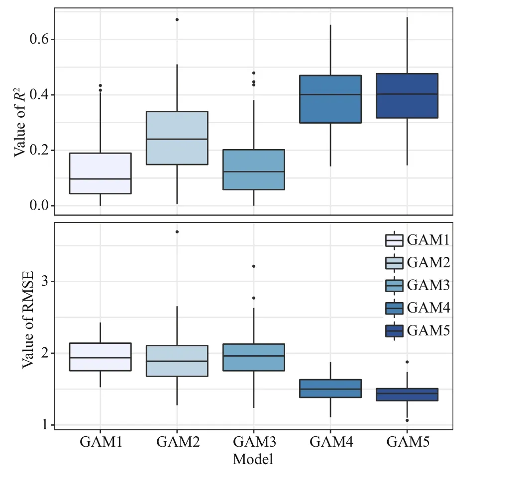
Fig.8 R2 and RMSE resulted from 100 times crossvalidations of five generalized additive models(GAMs)

The predictive ability of habitat models could be limited by the explanatory variables collected from diff erent sources (Dambach and Rödder, 2011). The spatial distribution of prey is one of the factors driving the distribution of predators through bottom-up eff ect(Bi et al., 2011; Zerbini et al., 2016). Understanding of the spatial relationship between fish and their prey can help to discover the hot spots of feeding and the spatial distribution of predators (Lasley-Rasher et al.,2015). The spatial overlap between predators and their prey species can improve the feeding effi ciency and reduce the energy loss of foraging. The availability of prey species can also compensate for some unfavorable factors, such as the eff ects of temperature and salinity (Youcef et al., 2013). That is probably the reason why prey species is one of the important drivers for the distribution ofJ. belangerii. Lack consideration of predator-prey interactions may lead to biased predictions of species distributions.

Previous study revealed the necessity to incorporate SAC into habitat models via spatial methods when significant SAC was detected in the residuals (Wu et al., 2009). We found that the GAMs incorporating SAC showed substantial reductions in residual spatial autocorrelation (Supplementary Fig.S1). Through the addition of SAC in GAMs, an extra part of the variance was explained and more accurate estimates of regression coeffi cients were provided (Jewell et al.,2007; Wu et al., 2009). This study showed that GAMs that ignore SAC in ecological data might misestimate the spatial distribution of target species, which may result in improper management recommendations.

Information on the spatial distribution of target species is important for the management and monitoring of fishery resources. The development of marine protected areas (MPA) and ecosystem-based fishery management (EBFM) need to assess the temporal and spatial distribution of target species and their relationship with environmental factors,particularly in areas under severe climate changes. In addition, fisheries managers wish to obtain reliable species distribution map to identify essential habitats for species (Vinagre et al., 2006; Chang et al., 2012).However, EBFM is often hampered by the lack ofinformation on habitats and distribution ofimportant species (Pikitch et al., 2004). Understanding the spatiotemporal dynamics of species distribution and its relationship with environmental variables is critical for the implementation of EBFM and the habitat assessment (Liu et al., 2019). Neglecting the eff ects of biotic variables and SAC may result in biased habitat models. This study showed that PCA-based GAM incorporating SAC of target species could improve the performance of habitat model, which can better serve management strategies and identify Essential Fish Habitats (EFH) (Xue et al., 2018).

The lack of field observations of prey species and spatial autocorrelation of predator could reduce the accuracy of SDMs (Wu et al., 2009; Xue et al., 2018).Based on our findings and previous study (Xue et al.,2018), the habitat models of marine organisms should monitor both predators and their important prey species. Further investigation of the interaction between predators and prey is needed in future. The diff erences in the growth and dynamics of both predators and prey should also be fully taken into account to improve the accuracy of habitat models,which will help to provide more support for the conservation and sustainable utilization of fishery resources. In addition, the impact of climate change on marine life in small-scale sea areas has received increasing attention from researchers (Bates et al.,2018). The spatial-temporal distribution of target species over diff erent life history stage under climate change should also be considered in future work.

5 DATA AVAILABILITY STATEMENT

The data generated or analyzed in this study are available from the corresponding author on reasonable request.

6 ACKNOWLEDGMENT

We are grateful to many colleagues and graduate students for assistance in sample collection and analyses in laboratory and in the field. We also thank two anonymous reviewers for their valuable and constructive comments on this paper.