Modeling and parameter identification of linear time-varying systems based on adaptive chirplet transform under random excitation
2021-05-14JieZHANGZhiyuSHILirongLI
Jie ZHANG, Zhiyu SHI,*, Lirong LI
a State Key Laboratory of Mechanics and Control of Mechanical Structures, Nanjing University of Aeronautics and Astronautics, Nanjing 210016, China
b Shanghai Aircraft Customer Service Co., Ltd., Shanghai 200241, China
KEYWORDS Acceleration response;Chirplet transform;LTV systems;Random excitation;System parameter identification
Abstract In this paper, a time-frequency algorithm based on adaptive chirplet transform for parameter modeling and identification of Linear Time-Varying (LTV) systems under random excitation is presented.It is assumed that the solution of responses of LTV structures is expressed as the sum of multicomponent Linear Frequency Modulated(LFM)signals in a short-time.Then the measured acceleration response is used to perform the adaptive chirplet transform,in which an integral algorithm is employed to reconstruct the velocity and displacement responses.The vibration differential equation with time-varying coefficients is transformed into a simple linear equation.Furthermore,for systems under random excitation,the input-output relation based on correlation function is also derived to estimate the parameters including physicals parameters and instantaneous modal parameters. The full procedure of the method is presented and validated by using simulated responses.The results show that the presented method is accurate and robust for various LTV systems under random excitation.
1. Introduction
Dynamic parameter identification of mechanical systems has a wide range of practical applications in engineering design,vibration testing, damage detection and health monitoring,etc. Classical vibration analysis based on system identification is usually divided into Experimental Modal Analysis (EMA)and Operational Modal Analysis (OMA). EMA is a useful technique to build vibration modal based on measured input and output data. However for most engineering structures(bridge,aircraft,space station,etc.),OMA is more convenient and feasible in application since it can identify modal parameters only from measured output data. Research work on OMAincludes various methods such as the random decrement technique, stochastic subspace identification, frequency domain decomposition method, autoregressive moving average methods, etc. Most of these approachesassume that dynamics parameters of these analyzed structures should be Linear Time-Invariant (LTI). With the research on high level technology, some large scale structures with time-varying parameters have appeared, such as flight rockets, supersonic and hypersonic vehicles, rotating machineries, etc. The theoretical solution and modeling methods based on classical vibration analysis have fallen short of application for these structures. Consequently, research on Linear Time-Varying(LTV) systems has attracted wide attention and various methods have also been developed and investigated for the modeling and identification of LTV systems.
For the vibration analysis of LTI systems, Frequency Response Functions (FRF) in frequency-domain or Impulse Response Functions (IRF) in time-domain can be obtained directly by solving the LTI vibration differential equations.Based on these response functions, classical identification approaches can be performed and generally belong to two categories:time-domain methods and frequency-domain methods which rely on Fourier Transform (FT). It is well known that time-varying parameters lead to non-stationary structural response. Theoretically, analytical solution for response of LTV systems cannot be obtained directly, especially for structures under random excitation. Thus traditional time-domain model and FT are not suitable to process the non-stationary response data of LTV systems,time-varying models(for example, time-varying vibration differential equation, state-space model and time series model) and Time-Frequency Analysis(TFA) tools (for example, Hilbert Transform (HT),Wavelet Transform(WT),etc.)are further introduced into parameter identification of LTV systems. LTV structural identification methods may be primarily classified as time-domain methods and Time-Frequency-domain (TF-domain) methods.
For the vibration analysis in time-domain, second-order vibration differential equation,state-space model and time series model are the most widely used models to express LTV structures.By treating a LTV structure as a LTI system within a short time interval, least squares method, Singular Value Decomposition (SVD), Kalman filter, etc. can be directly applied to obtain the solution of LTV systems. Ghanem and Romeopresented a wavelet-based identification method,which transforms a differential equation into a wavelet expansion form and identifies the parameters using the wavelet Galerkin approach. Wang et al.presented a moving window second order blind identification method for OMA of slow linear time-varying structures, by which the displacement response could be expressed in modal coordinates to solve the time-varying differential equation, and each of order modal parameters could be identified. Liuproposed a subspace-based identification technique and used eigenvalues of the estimated transition matrices to characterize the dynamic properties. The subspace is constructed by the singular value decomposition (SVD) which costs too much computational time. Authorsfurther presented an improved algorithm using the combined measurements of DVA obtained from only one experiment to overcome such drawback. Pang et al.utilized the Projection Approximation Subspace Tracking(PAST)technique instead of the SVD.Ni et al.proposed a recursive tracking approach based on RPBSID algorithm for the manipulator inertia parameter identification. Meanwhile,in order to process non-stationary responses of time-varying structures, many approaches were also proposed based on the Time-dependent Autoregressive Moving Average(TARMA) model.The TARMA model can be utilized as an efficient tool to reveal the dynamic characteristics of nonstationary signals due to its simplicity and effectiveness. Spiridonakos and Fassoispresented an adaptable functional series TARMA model for non-stationary signal modelling,which employs the B-spline function to model the TARMA coefficients adaptively and structurally. Li et al.developed a Bayesian estimator based on time-dependent autoregressive model, which has the advantage of supplying the uncertainty with the creditable interval estimation. As mentioned in the above literature review, one of the main procedure is to adopt the theory of time-freezing,that is to say,the time-varying system is expressed as a LTI model at each freezing time,then the parameters can be estimated using LTI identification methods.But in order to be close to a LTI system, the time step of system modeling must be small, which makes the methods computationally expensive and only applicable to slow-varying systems.
Furthermore,TF-domain signal processing tools have been more extensively studied, i.e., HT,Gabor transformand WT,since the response of LTV systems is a typical nonstationary signal which needs to be processed by TFA tools.Meanwhile, TFA tools become effective in solving timevarying equations with the development of TF theory. In Ref. 21, Shi et al. developed an algorithm using HT and EMD to decompose a general signal into IMFs and then track the variations of LTV MDOF systems. Further, a waveletbased state-space methodfor LTV systems identification was proposed by Xu et al. Ref. 23 proposed a continuous wavelet-based technique for identification of instantaneous modal parameters of time-varying structures. Staszewski et al.used the wavelet-based FRF for modal identification of time-variant system.Ref.25 addressed a TF decomposition approach based on Empirical Wavelet Transform to identify the instantaneous frequencies of a time-varying two-storey shear type building.
Among these methods,WT are the most widely used methods.However they are insufficient to provide a TF representation with high resolution due to their inherent restrictions.They are established on the assumption of the considered signal being piecewise stationary in a short time interval.It means that they essentially use horizontal lines to approximate the Instantaneous Frequency(IF)feature.This is also the inherent reason why the theory of time-freezing should be adopted in most identification methods. To improve the performance of TFA tools, a general TFA tool with adaptive basis functions should be explored. According to the dynamic behaviors of strongly LTV systems, the vibration responses should be frequency modulated rather than piecewise stationary in a short time interval, which gives a novel idea for the expression of the vibration responses. Although the analytical expression of the nonstationary vibration responses of LTV mechanical systems cannot be got directly, it should be approximately fitted with multicomponent Linear Frequency Modulation(LFM)signalsin a short time interval.Fortunately,the Chirplet Transform (CT) recently designed in Ref. 27 made it possible to create a concentrated TF representation for a monocomponent LFM signal. Yu and Zhoudeveloped an adaptive algorithm named GLCT to search the best chirp rate for multicomponent LFM signals.The work in Ref.29 utilized the Polynomial Chirplet Transform (PCT) to process nonstationary signals and perform parameter estimation for nonlinear systems. Chen and Yuproposed a method based on multi-scale chirplet sparse signal decomposition to identify a single degree of freedom system. Therefore, adaptive CT is particularly suitable to perform TFA of non-stationary response signals. By introducing a demodulated operator,it produces a more accurate IF estimator and retains the signal reconstruction ability.
It can be seen from the above analysis that a novel algorithm for solving time-varying differential equations may be provided by decomposing vibration responses into a linear combination of basis functions of chirplet. Using this algorithm, we can transform the differential equation of LTV vibration systems into a linear equation and establish a linear model between time-varying parameters and input-output data. In order to implement this algorithm, we need to solve two key problems firstly. The first one is constructing a LTV model only using acceleration response and transforming the differential equation into a linear equation, since acceleration response is more convenient to be measured than other responses. The other is to derive the stochastic input-output relation. To solve the first problem, we propose an integral algorithm based on CT, in which only structural acceleration response is used to reconstruct the velocity and displacement responses.For the solution of another problem,the ambiguity function provides a novel idea to obtain the correlation function of LFM signals. The correlation function is widely used in the analysis of LFM signals,especially in estimation of modulation signals.It is worth noting that the response signals of a LTV model are assumed to be the sum of multicomponent LFM signals in a short-time. As analyzed in Refs. 33-35, the ambiguity function can reflect the correlation of LFM signal in time-domain. Thus, it makes it possible to get the relation between correlation functions and time-varying parameters.
A new algorithm for random vibration analysis only using acceleration response is presented in this paper,with a focus on solving dynamic equation with time-varying parameters and getting the relation between time-varying parameters and input-output data. The rest of the paper is organized as follows: The theory of chirplet integral is briefly introduced in Section 2. Stochastic vibration model with time-varying parameters, along with a brief outline of correlation function of LFM signals,is presented in Section 3.Then the established linear model can be used to identify time-varying parameters.Section 4 shows a series of numerical simulation examples to illustrate the performance of identification for various timevarying cases. Finally, Section 5 provides conclusions on the proposed method.
2. Theoretical analysis for chirplet transform and integral algorithm
2.1. Adaptive chirplet transform
The CT is a TFA tool for generating TF representation of a monocomponent LFM signal. Consider a monocomponent analytic signal with time-varying IF as


In Eq. (4), when demodulated coefficient c is consistent with ˙φ(t) of the analyzed signal, the CT amplitude will achieve the maximum, and then the better TF representation with high energy concentration will be obtained.
But for multicomponent signals with N components as follows

The IF feature of this signal cannot be known in advance,which leads to difficulty to determine the demodulated operator accurately.An adaptive approach in Ref.28 is to use a series of discrete demodulated operators c(t)to approximate the best demodulated operator. So a parameterαis introduced to characterize the parameter c(t), as

where Tand Fare the sampling time and sampling frequency in the short time interval, respectively. In a discrete way, the parameter α is divided into Nvalues on the TF plane from-π/2 to π/2, as
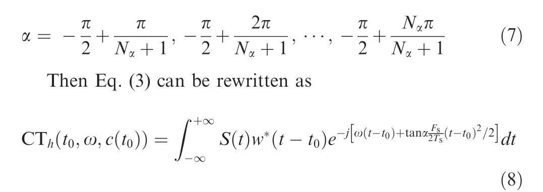
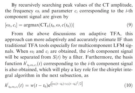
2.2. LTV model and integral algorithm
In engineering practice, it is more convenient to perform the measurement of acceleration response. Therefore, the integral algorithm based on CT is deduced only using the structural acceleration response and the velocity and displacement response signals are reconstructed by using this algorithm.
The parameter model of a LTV damped system with N degrees-of-freedom (dofs) is provided by the vibration differential equation


Meanwhile,according to the attenuation of basis functions,the following equation is given as
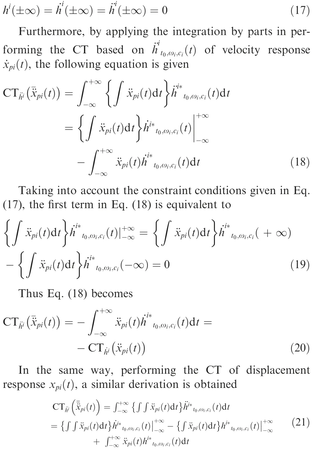
By virtue of Eq.(17),the first two terms in Eq.(21)is equivalent to

Fig. 1 Time domain waveform of basis functions.

Each monocomponent signal of velocity and displacement response are reconstructed by

3.Modeling and parameter identification of LTV systems under random excitation
For most time-varying structures in engineering practice,structural excitation is usually random and unmeasurable. In this section,by adopting ambiguity function theory and mathematical statistics theory, a time-varying model based on correlation function is established and from which parameters are extracted.By using the chirplet integral algorithm,the velocity and displacement responses are reconstructed.Then the vibration differential equation with time-varying parameters is transformed into a simple linear equation:

Express the responses as superposition of multicomponent LFM signals:

It is worth noting that Eq. (29) is a linear equation which can be used to express the relation between time-varying parameter matrix and input-output data. If the excitation u(t ) is known, we can use this equation to identify timevarying parameters. However, u(t ) is random and unmeasurable for most LTV structures,which makes it necessary to perform the correlation analysis for input and output signals.
3.1. The ambiguity function of LFM signals

The calculation of cross-correlation functions between y(t )and y(t )is a complicated mathematical problem,but it can be proved that, when Δω is not a smaller value compared with carrier frequency ω, the following equation can be obtained:

3.2. Random modeling and parameter identification
By adopting ambiguity function theory and mathematical statistics theory, a time-varying model based on correlation function is established and from which time-varying parameters are extracted. Assuming that the excitation in Eq. (29) is a stationary Gaussian white-noise with zero mean,the correlation function of excitation is given by

Using the operator in Eq. (34), the correlation function matrix of input is given by

Substituting Eqs. (36) and (37) into (35), a time-varying model can be formulated as

Fig. 2 A time-varying three-storey shear type building.
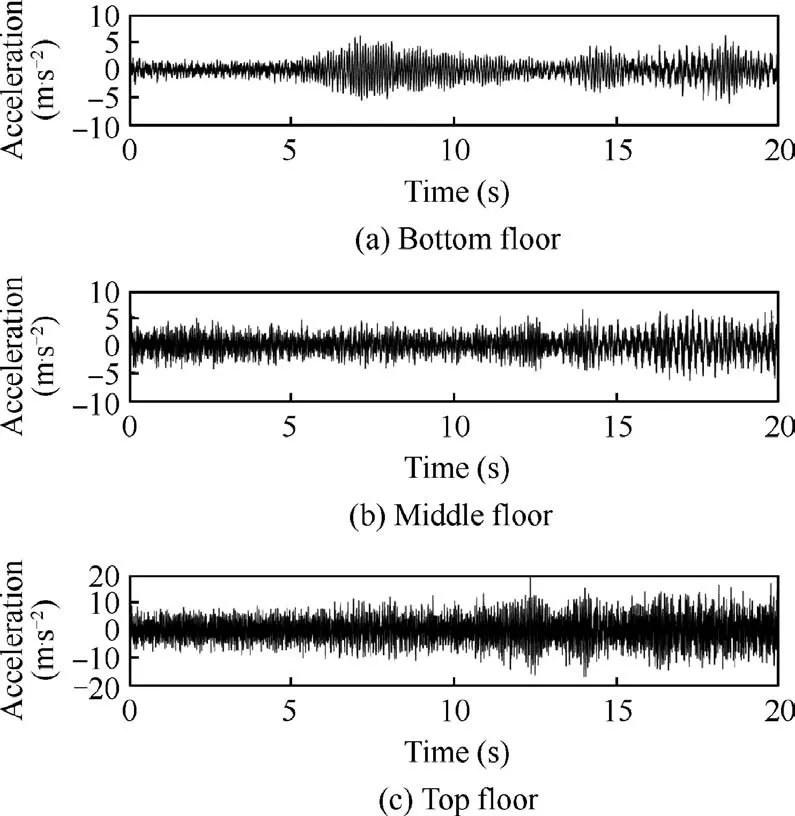
Fig. 3 Acceleration response at bottom floor, middle floor, and top floor.

4. Simulation example
In order to validate the proposed method, a time-varying three-storey shear type building, as displayed in Fig. 2, is simulated as a numerical example. In this section, the structure is subjected to external excitation of random Gaussian white noise series.The time-varying structure has three initial masses of m=2.0×10kg at the bottom floor,m=1.0×10kg at the middle floor, and m=5.0×10kg at the top floor. Three initial stiffness coefficients k=k=k=4.0×10N·m are assumed for this structure. Initial damping coefficients are set as c-=c=c=8.0×10N·s/m. The sampling frequency and sampling time of the analysis is 1024 Hz and 20 s,respectively.

Fig. 4 Reconstructed velocity and displacement responses at bottom floor, middle floor, and the top floor.

Table 1 Error analysis of integral algorithm.
To simulate the time-varying dynamic characteristics of the structure, various variations in time of physical parameters,including smooth variations,periodic variations and quadratic variations, are employed to model the structure.
Case 1: Mass variations.
In this case, it is assumed that the stiffness coefficients are time-invariant.The mass and damping variations are given by

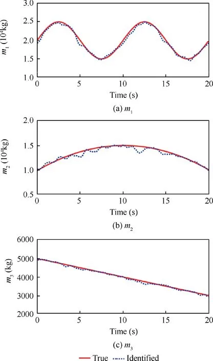
Fig. 5 Identified results of mass coefficients via the proposed method.
The excitation applied at all three floors is a random white Gaussian force with zero mean and 10variance. The Newmark method is used to calculate the acceleration response due to the random force.The calculated response data at three floors is shown in Fig.3.Then the proposed integral algorithm can be performed using the acceleration response to reconstruct the velocity and displacement responses which are shown in Fig. 4. Fig. 4 also provides a comparison between true responses and reconstructed responses. It is shown that the proposed algorithm makes a good performance of reconstructing signals.


Fig.6 Identified results of damping coefficients via the proposed method.

Fig.7 Estimated instantaneous frequencies based on eigenvalue decomposition of identified physical parameter matrix.

Fig. 8 Estimated instantaneous damping ratio based on eigenvalue decomposition of identified physical parameter matrix.
In order to further demonstrate the performance of integral algorithm, mean squares error (MSE) is used to calculate the reconstruction error. MSE is defined as follows:in which Nrepresents the number of sampling points,s and srepresent true and reconstructed signal respectively.The calculated MSE values are listed in Table 1. From these values, the accuracy of reconstruction algorithm is verified.
Then according to the time-varying linear equation in Eq.(39), physical parameters can be identified. The identified results of time-varying mass coefficients and damping coefficients are shown in Figs. 5 and 6, respectively. The estimated instantaneous frequencies and damping ratios can be observed from Figs. 7 and 8, respectively. These results show that the algorithm can well track various variations in time of both physical parameters and modal parameters.
However,it can also been discovered that relative errors of identification results in Figs.6 and 8 are great.This is because damping coefficients in physical parameter matrix as shown in Eq. (39) are smaller values compared with mass coefficients and stiffness coefficients, so identification error of damping coefficients is larger than other errors when physical parametermatrix is identified as a whole. In addition, identification results of parameters of nonlinear variation are not as good as that of linear variation.
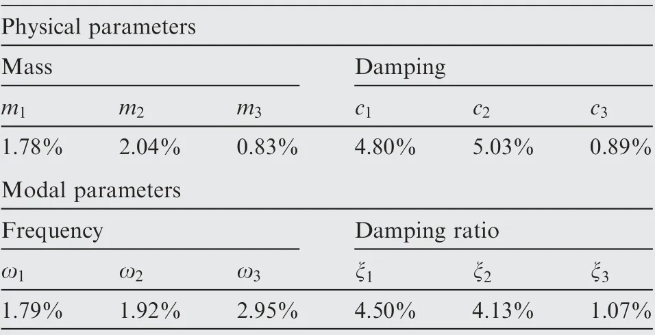
Table 2 Error analysis of identification results.

Fig.9 Identified results of stiffness coefficients via the proposed method.

Fig. 10 Estimated instantaneous frequencies based on eigenvalue decomposition of identified physical parameter matrix.

Fig. 11 Estimated instantaneous damping ratio based on eigenvalue decomposition of identified physical parameter matrix.

Table 3 Error analysis of identification results.
To further investigate the performance and reliability of the proposed method, an error index is defined as mean absolute percentage error over the total sampling time to quantify the accuracy of the identified results:


Case 2: Stiffness variations.
In this case, it is assumed that the mass and damping coefficients are time-invariant.The stiffness variations are given by

The excitation applied at all three floors is the same as the random excitation in Case 1. The same procedure as above is followed to identify the time-varying parameters only using the acceleration response. The identified results of time-varying stiffness coefficients are shown in Fig. 9, and the estimated instantaneous frequencies and damping ratios are depicted in Figs. 10 and 11, respectively. In the same way, we perform the error analysis to show the performance and reliability of the identification method using the error index in Eq. (41).The result of error analysis is shown in Table 3. Generally, it can be concluded that the proposed method can well model the LTV structure, as well as identify structural parameters.
5. Conclusions
In this paper,a novel time-frequency algorithm based on chirplet integral for the time-domain representation of responses of LTV systems under random excitation is presented. With this method, we can only using the measured acceleration response to reconstruct velocity and displacement responses,thus transforming the time-varying differential equation into a linear equation. The complex inverse problem for LTV systems can be solved and time-varying parameter can also be identified. Since only random acceleration response data is used in the identification procedure, this is very convenient for the vibration testing of practical engineering structures.The full procedure of the method is presented and validated by using simulated responses. The results show that the presented method is accurate and robust for various LTV systems under random excitation.
Declaration of Competing Interest
The authors declare that they have no known competing financial interests or personal relationships that could have appeared to influence the work reported in this paper.
Acknowledgement
sThis work was funded by the National Natural Science Foundation of China (Grant No. 11172131 and 11232007) and the Priority Academic Program Development of Jiangsu Higher Education Institutions.
杂志排行
CHINESE JOURNAL OF AERONAUTICS的其它文章
- Time delay compensation in lateral-directional flight control systems at high angles of attack
- Dual stability enhancement mechanisms of axial-slot casing treatment in a high-speed mixed-flow compressor with various tip clearances
- Development cost prediction of general aviation aircraft using combined estimation technique
- Improvement on shaped-hole film cooling effectiveness by integrating upstream sand-dune-shaped ramps
- An experimental method to obtain the hard alpha anomaly distribution for titanium alloy aeroengine disks
- Vibration analysis and control technologies of hydraulic pipeline system in aircraft: A review
