A simplified approximate analytical model for Rayleigh–Taylor instability in elastic–plastic solid and viscous fluid with thicknesses∗

Xi Wang(王曦), Xiao-Mian Hu(胡晓棉), Sheng-Tao Wang(王升涛), and Hao Pan(潘昊),2,†

1Institute of Applied Physics and Computational Mathematics,Beijing 100094,China

2Center for Applied Physics and Technology,Peking University,Beijing 100871,China

Keywords: Rayleigh–Taylor instability,viscosity,plasticity,thicknesses effects

1. Introduction

The Rayleigh–Taylor instability(RTI)is ubiquitous when denser material lays above lighter one in gravitational field,or denser one is accelerated by the lighter one.[1–6]RTI in solids is dramatically determined by the nonlinear constitutive relation of elastic–plastic(EP)mechanical properties. Barnes’pioneer experiment performed that the perturbation growth was apparently governed by yield strength of EP solid.[7]In addition,the instability evolution is dependent on both the perturbation wavelength and the initial perturbation amplitude of the interface, which was noticed by Drucker[8]and subsequently confirmed by Barnes’ later experiment.[9]The complex mechanical behaviors of RTI in solids are far from sufficiently understood for present.

The RTI in solids plays a great role in many physics research area, such as of relevance in geophysics, astrophysics,high energy density physics, and the inertial confinement fusion(ICF).[10–16]The problem especially causes attention because it can be a test experimental tool to evaluate yield strength and other mechanical properties of solid slab under extremely high strain and high strain rate conditions.[10,17–19]Furthermore, the solid accelerated by the melted metal layer generates RTI phenomena in experiments, such as, magnetically imploded liners[12,20,21]and the Laboratory Planetary Sciences experiment.[22–25]The EP mechanical transition of solid, viscosity of melted metal, thicknesses, and densities of two materials in the realistic experiments are usually concurrent and unavoidable. Those physical behaviors boost the complication of the theoretical analysis of RTI evolution.

For the purposes of comprehending the RTI in solids,several theoretical description models for the instability evolution have been developed, including the model based on energy balance, the normal modes method, the model based on the Newtonian second law,and the velocity composition method.

A firstly model based on energy balance was developed by Miles,[26]then followed by Robinson and Swelge,[27]for EP solid slab and vacuum interface with realistic physics meaning, but lacking sufficiently accuracy and underestimating the growth rate[28]and difficult to contain other effects such as viscosity,surface tension,and thicknesses of two materials.

The traditional normal modes method has been only applied into perfectly elastic solids[3,29,30]and it is too mathematically complex to treat the strength behavior of solid material to obtain analytical results. Although, inspired by Mikaelian,[31]Colvin replaced surface tension term with a shear modulus dependent term in elastic regime and expressed yield strength as effective lattice viscosity after plastic transition,[17,19]this method is still controversial in interpreting experiments.[32,33]

Furthermore,a model based on the Newtonian second law can simply consider different forces acting on the perturbed interface,such as surface tension,viscosity,elasticity,plasticity,etc.[34–38]Yet, the model is merely established for two semiinfinite thicknesses media.

With the velocity composition, Sun improved the accuracy of approximate solutions of the growth rates for a semiinfinite solid–solid interface and solid–fluid interface but with the assumption of elastic solid.[39]Besides,Sun only showed the dispersion relation of the elastic solid slab with arbitrary thickness accelerated in a semi-infinite rarefied inviscid region.[39]In addition, Piriz obtained the stability boundaries by using the Helmholtz decomposition in the elastic phase,following Drucker[8]and the method of the limit analysis to treat rigid-plastic phase.[40]But, only solid accelerated by semiinfinite idea fluid is discussed. The composition method has not been performed to solid slab with plastic mechanical properties leading to different methods used in elastic and plastic regimes.

The representative RTI system,that finite-thickness solid with EP properties is accelerated by finite-thickness fluid with viscosity,is rarely studied by the previous theoretical models,which prevents the thorough interpretations of RTI in solids.Therefore, RTI between finite-thickness EP solid and finitethickness viscous fluid,which is much closer to experimental conditions, is concentrated on. The goal of the present work is to illustrate a simplified approximate analytical method for RTI with relatively easy mathematical treatment and the convenient extension potential.

In this study, a simplified RTI linear analysis model for EP solid and viscous fluid both with arbitrary thicknesses and densities is performed. The primary idea of the model with the irrotational velocity potentials, which were used in fluids,[41]is presented and the reasonability for the simplification is shown in Section 2. In Section 3,previous approximate dispersion relation with viscosity and surface tension in finitethicknesses fluids is obtained again by the model. Then, in Section 4, the analytical equation of perturbation amplitude evolution for EP solid and viscous fluid both with arbitrary thicknesses and densities, that can cover the early results of semi-infinite cases which were in excellent agreements with two-dimensional simulations,[36–38]is achieved. Moreover,the corresponding growth rate (in Subsection 4.1) and instability boundaries(in Subsection 4.2)are derived. The effects of thicknesses of two materials are discussed in the results in Subseection 4.3.

2. Analytical model

Figure 1 gives RTI features of two immiscible materials with the heavier one of density ρ1lying above on the lighter one of density ρ2at constant accelerator g which has opposite direction to y axis. Materials 1 and 2 have the thicknesses of h1and h2respectively. The materials are separated by y=0 at initial moment.

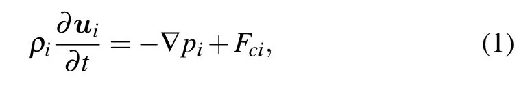
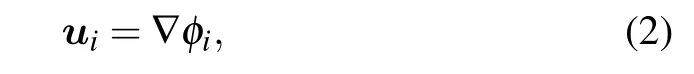
For the RTI system with viscosity, surface tension, elasticity, the forces acting on the interface will depend on the perturbed velocity field determined by the momentum conservation equations. The velocity field can be decomposed into irrotational and rotational parts expressed by the velocity potentials and the stream functions as Bellman and Pennington did.[41]Because the forces at the interface generate the rotation of the flow field, the velocity decomposition method is hard to directly extend to the plastic regime of solid to obtain analytical results due to the nonlinear constitutive relation with EP transition. In order to deal with the complex RTI system which is closer to realistic situation, a simplification is made below.

In this work, the velocity field of the flow is assumed to be irrotational and expressed by the velocity potentials. The irrotational flow simplification is reasonable as mentioned in Ref. [42], that the vorticity generated by the forces acting on the interface only affects the velocity field for the wave number smaller than the associated vorticity mode,but RTI is rather insensitive to the velocity field for the smallest values of the wave number and the interface approaches the classical behavior. Besides, it needs to be emphasized that, with the perfect plastic assumption,the displacement field must be irrotational.[43]Although the accuracy may be reduced by the simplification, it is possible to deal with more complex situation with effects of EP transition, viscosity, and arbitrary thicknesses of two materials simultaneously. With the approximation, the analytical results can be achieved including the evolution of the perturbation amplitude, the growth rate, and the stability boundary for the interface of arbitrary thickness EP solid and arbitrary thickness viscous fluid in Section 4.The analytical expressions can cover the Piriz’s semi-infinite results which are in excellent agreement with two-dimensional simulations.[36–38]

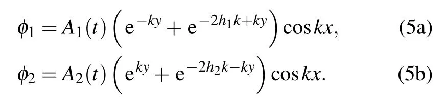
φifor two materials with finite thicknesses have the following forms:[39,44]

where Ai(t) and Bi(t) have the form ∼entwhere n is the growth rate. By combining the boundary conditions at y=h1and y=−h2when both materials are attached to a rigid side wall,

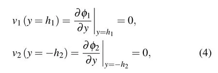
where ν1and ν2are the vertical velocities of materials, the velocity potentials turn into

The initial interface y=0 is perturbed by infinitesimal disturbance

where k=2π/λ is the wave number of the perturbation surface in x direction,λ is the perturbed interface wavelength,and ξ(t)is the perturbation amplitude. Similarly to the way done in Ref.[39],by integrating Eq.(1)from y=0 to the interface y=η(x,t)and substituting velocity expression Eq.(2)into the integrated equation,the formulation of pican be written as

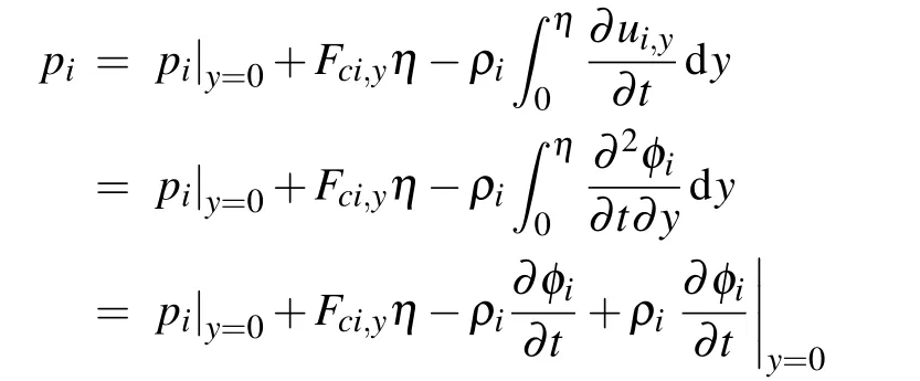
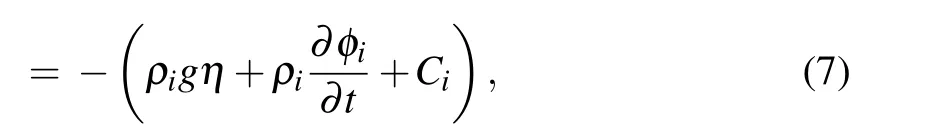
At the initial state we have y=η(x,0)=0 and the interface is in approximate equilibrium,then C1=C2can be obtained.

At the interface, the continuity of velocities and force equilibrium along the y direction need to be satisfied at any instantaneous time. The interface motion can be controlled by the normal velocity continuity equation

and the normal force equilibrium

3. Finite-thicknesses fluids with viscosity and surface tension

The model is first applied to the RTI system of two finite thicknesses viscous fluids with surface tension to claim the reasonability of the methodology.

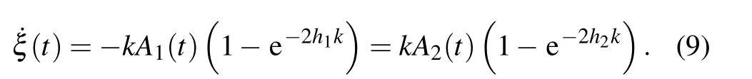
Based on the velocity continuity at the perturbation interface in Eq.(8a),the correlations of the interface amplitude ξ(t) and the velocity potential factors A1(t) in Eq. (5a) and A2(t)in Eq.(5b)can be obtained

And,there is the normal force equilibrium at the material interface according to Eq.(8b),i.e.

For the Newtonian fluid at each side of the interface,the strain rate tensors are shown below:

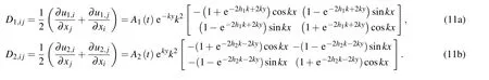
Then,because the deviatoric stress tensors have the forms of

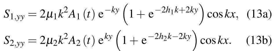
where µ1and µ2are the dynamic viscosities of fluids 1 and 2 respectively,we can get the vertical components of stresses produced by viscosity:

The effect of surface tension at the interface is performed by the Young–Laplace equation

where Tstis the surface tension coefficient and R is the local curvature radius which has the expression of

By substituting Eqs. (7), (13a), (13b), and (14) into Eq. (10), we obtain the motion equation of the interface amplitude ξ(t)at y=0

whose dispersion relation of the growth rate is exactly the same as the approximate result of the dispersion relation formula Eq.(25)in Ref.[31]performed by Mikaelian who started from the general eigenvalue equation[46]by the classical normal modes analysis and then substituted the exact eigenfunctions for the inviscid case directly.

4. Solid slab and finite-thickness fluid interface

Next, material at y > 0, below which viscous fluid of finite-thickness domain is still maintained, is changed to be solid slab with thickness h1. The relations of the interface amplitude and the velocity potential factors can be derived as the similar way by combining the interface velocity continuity principal. The expression is uniform with Eq.(9).

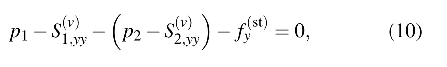
By keeping equilibrium of the forces at the material interface,we have

For a linear elastic solid(a Hookean solid),[47]the deviatoric stress tensor can be written as

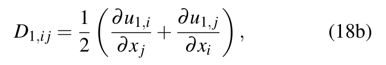
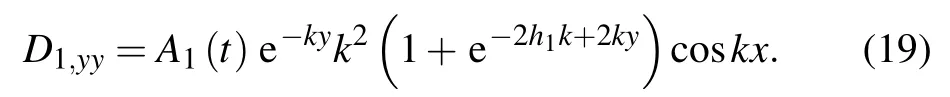
where G1is the shear modulus of solid slab. By evaluating the velocity potential Eq.(5a),the rate of deformation tensor D1,ijin the y direction becomes

By giving the interface profile η(x,0)=ξ0coskx at initial time and integrating Eq.(18a)with Eq.(9),we obtain the deviatoric stress tensor

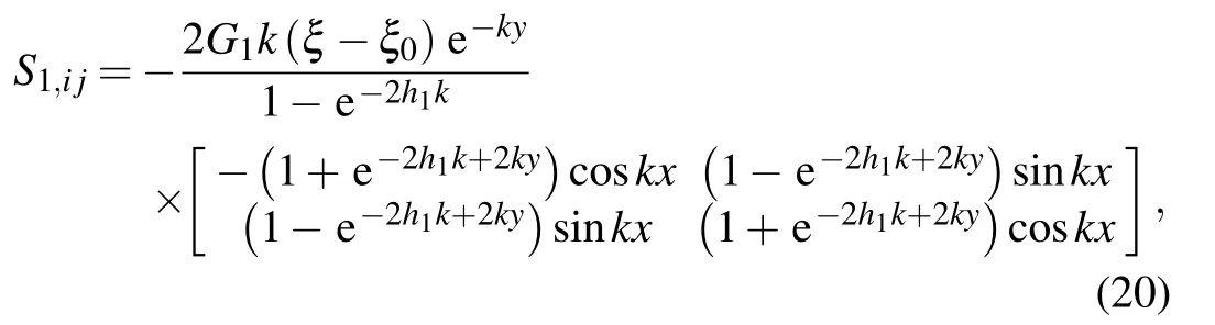
and the vertical component in the elastic regime is

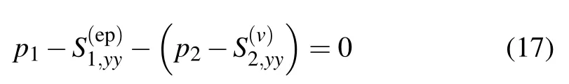
Therefore,after substituting Eq.(21)into Eq.(17),we have

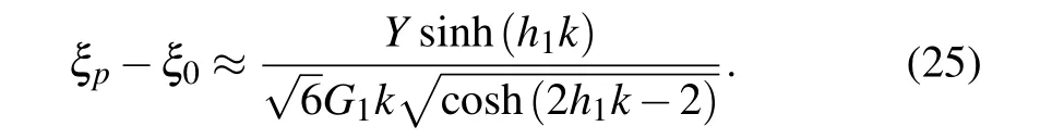
When the effective stress arrives at the yield strength Y,

i.e.,

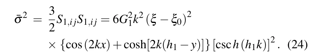
the solid slab will transient from elastic to plastic regime. By substituting the deviatoric stress tensor Eq.(21)into the effective stress,we have the specific expression below:

Thus,by combining the elastic branch in Eq.(22),the amplitude growth equation for EP solid slab accelerated by finite thickness viscous fluid is

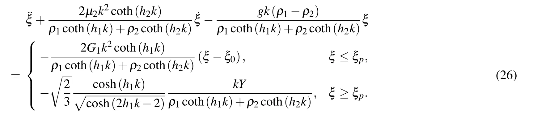
The motion equation can describe the solid/fluid RTI system with arbitrary Atwood number, arbitrary thicknesses of both materials, dynamic viscosity, shear modulus and yield strength. Compared to the two fluids RTI case of Eq. (16)which is irrelevant with ξ0, the evolution of interface is controlled by the initial perturbation amplitude ξ0that is typical characteristic in solid which is found by Drucker[8]and confirmed by Barnes’experiment.[9]Furthermore,the thicknesses multiplied by wave number as a factor act on the densities of both mediums that will influence the perturbation growth rate and instability boundary as shown below.

When the interface of semi-infinite solid is accelerated by rarefied inviscid gas,i.e.,ρ2=0 andµ2=0,the motion equation turns into:

Equations(27)and(28)whose analytical instability boundary results showed excellent agreements with numerical simulations were previously obtained by the method established by Piriz.[36–38]

4.1. The dispersion relations

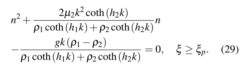
From the amplitude evolution of solid slab and finitethickness fluid interface in Eq. (26), it is convenient to obtain the analytical expression of the dispersion relation for the growth rate n for the plastic regime:

Here,the dimensionless growth rate σ,wave number κ,thickness and viscosity are introduced

and the equation for the dimensionless growth rate σ is

where AT=(ρ1−ρ2)/(ρ1+ρ2).

4.2. Stability boundary

Following the method in Refs. [37,38], the steps of deducing stability boundary are described below.

By introducing the following dimensionless variables:

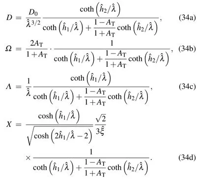
the motion Eq.(26)reads

where the symbols are defined as follows:

In addition,for the elastic–plastic transition,we have

and the corresponding initial conditions are

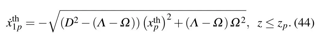
For the domain of z ≤zpand by introducing the transformation of

the first branch of Eq.(33)can be transformed into

and the initial conditions are

By integrating Eq.(39)for the first time with the initial conditions,we have

With the condition of

Similarly,with the transformation of

in the z ≥zpdomain, the second branch of Eq. (33) can become

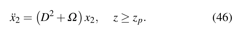
Combining the initial conditions

and performing integration once of Eq.(46),we obtain

As equation(37)must be satisfied on the stability boundary,it has

with the second branch of Eq. (33) and the derivative of Eq.(45). Thus,equation(48)reads

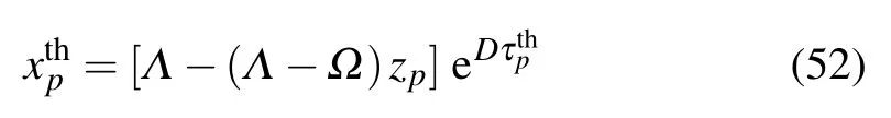
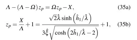
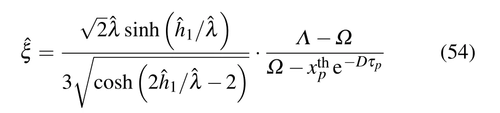
from Eq. (37). Then, according to the expression of zpin Eq.(35b),the instability threshold can be derived to be

which can be rewritten as

4.3. Results and discussions

4.3.1. Growth rate

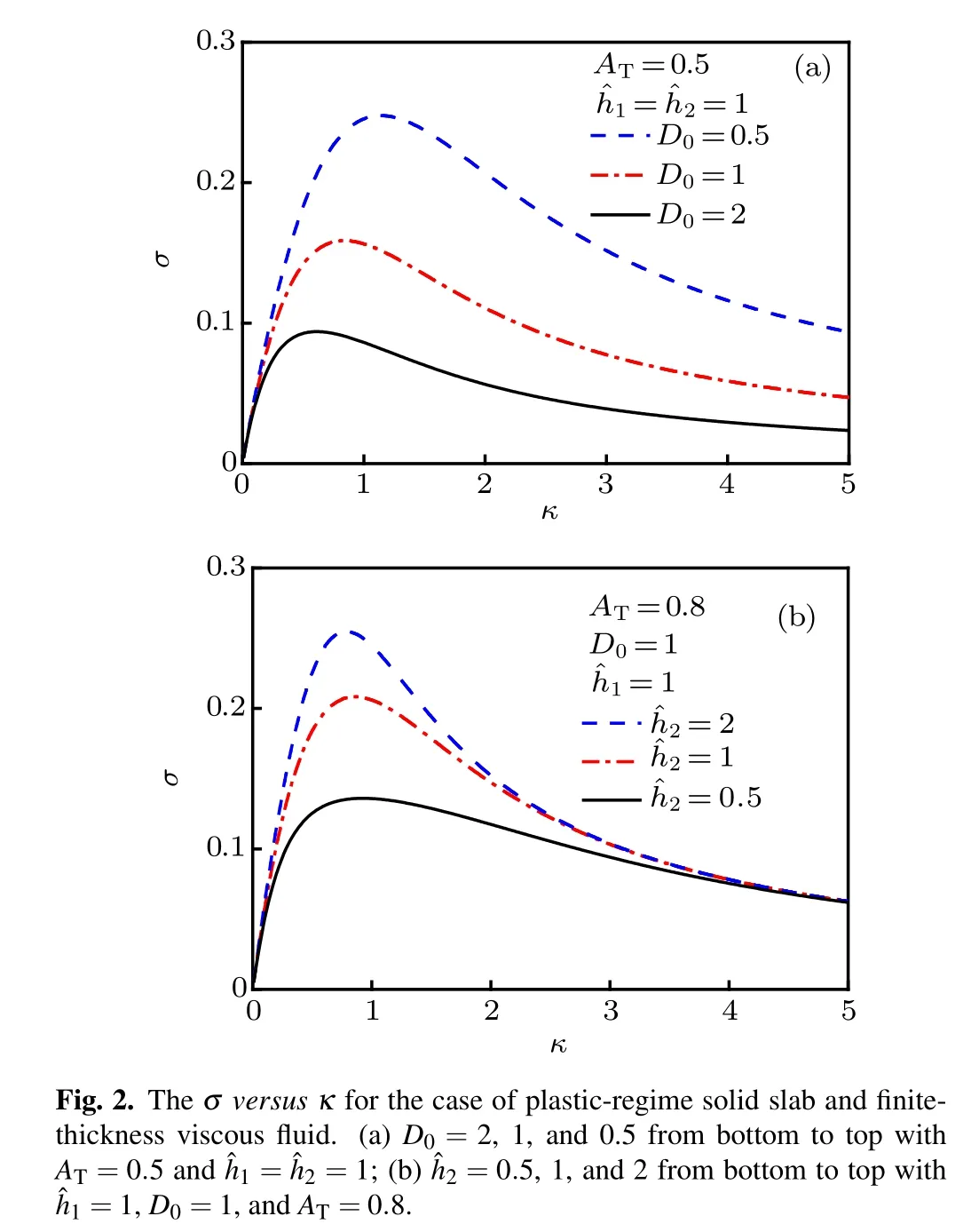
The dimensionless growth rate σ(κ)in the plastic regime is determined by the dispersion relation Eq. (31) which is a quadratic polynominal formula and always has real root. In Eq. (31), the solid yield strength does not affect the growth rate because of perfectly plasticity assumption that the yield strength is irrelevant to the strain after EP transition. Only the viscosity effect D0of fluid is left.

4.3.2. Instability boundary

5. Conclusion

A simplified approximate theoretical model for linear RTI system between EP solid and viscous fluid both with arbitrary thicknesses is presented in this paper. The model is with irrotational assumption and the velocity field is expressed with the velocity potentials.Although the solid constitutive relation has nonlinear characteristic which leads to be incapable to obtain analytical solutions for RTI in solids with EP transition by the previous velocity decomposition method, the model with the simplification in this work can deal with the viscosity,EP transition, and arbitrary thicknesses of both materials simultaneously with reasonable accuracy. The model treats thicknesses effects with boundary conditions in the irrotational velocity potentials and treats surface tension,fluid viscosity,and solid EP mechanical properties based on the continuity of velocity and force equilibrium at perturbation interface.

Applying the model in the RTI system of finite thicknesses fluids with viscosity and surface tension, the previous approximate dispersion relation deduced by the normal modes method is obtained again. Moreover, the analytical expressions of the interface amplitude motion equation, the growth rate and the instability boundary for the EP solid slab and finite thickness viscous fluid system are achieved, which can cover the cases with semi-infinite thicknesses by one-degreeof-freedom model based on the Newton second law.

The present study shows that the thicknesses of two materials unavoidably affect the instability evolution and reveals several features about thicknesses effect on the RTI system.For the plastic solid and viscous fluid interface, the growth rate is sensitive to the thickness of fluid. In addition,the thicknesses and ATof two materials change the shape of the instability boundary and the stabilizing effect with increasing viscosity is stronger for low ATthan for high AT.