Understanding the Soil Temperature Variability at Different Depths: Effects of Surface Air Temperature,Snow Cover, and the Soil Memory
2021-04-20HaoxinZHANGNaimingYUANZhuguoMAandYuHUANG
Haoxin ZHANG, Naiming YUAN, Zhuguo MA, and Yu HUANG
1Key Laboratory of Regional-Climate Environment Research for Temperate East Asia, Institute of Atmospheric Physics,Chinese Academy of Sciences, Beijing 100029, China
2University of Chinese Academy of Sciences, Beijing 100049, China
3Laboratory for Climate and Ocean-Atmosphere Studies, Department of Atmospheric and Oceanic Sciences,School of Physics, Peking University, Beijing 100871, China
(Received 18 March 2020; revised 20 September 2020; accepted 24 September 2020)
ABSTRACT The soil temperature (ST) is closely related to the surface air temperature (AT), but their coupling may be affected by other factors. In this study, significant effects of the AT on the underlying ST were found, and the time taken to propagate downward to 320 cm can be up to 10 months. Besides the AT, the ST is also affected by memory effects-namely, its prior thermal conditions. At deeper depth (i.e., 320 cm), the effects of the AT from a particular season may be exceeded by the soil memory effects from the last season. At shallower layers (i.e., < 80 cm), the effects of the AT may be blocked by the snow cover, resulting in a poorly synchronous correlation between the AT and the ST. In northeastern China, this snow cover blockage mainly occurs in winter and then vanishes in the subsequent spring. Due to the thermal insulation effect of the snow cover, the winter ST at layers above 80 cm in northeastern China were found to continue to increase even during the recent global warming hiatus period. These findings may be instructive for better understanding ST variations, as well as land-atmosphere interactions.
Key words: soil temperature, surface air temperature, soil memory, snow cover, nonlinear causality analysis
1. Introduction
Soil temperature (ST) is a primary component of the thermal regimes of land and plays an important role in land-atmosphere interaction. Similar to the oceans, land areas can record their early anomalous conditions, which subsequently affect the heat exchange between the land surface and the overlying atmosphere, making ST an important climate indicator at seasonal time scales (Hu and Feng, 2004a,b). As early as in the 1980s, the winter ST was used to predict the precipitation during the flood season (Tang et al.,1982, 1987; Tang and Reiter, 1986). From then on, understanding the variability of ST has received increasing attention (Mahanama et al., 2008; Fan, 2009; Xue et al., 2012;Wu and Zhang, 2014; Yang and Zhang, 2015). Many different factors, such as the variations of solar radiation, precipitation, vegetation, and surface air temperature (AT), have been reported to be vital in modifying ST (Zhang et al.,2001; Beltrami et al., 2005).
It is well recognized that the ST is normally closely coupled with the AT, and their temporal variations often exhibit similar characteristics (Beltrami and Kellman, 2003;Hu and Feng, 2005; Chudinova et al., 2006). This similarity, however, largely depends on the magnitude of the soil heat flux and the surface sensible heat flux, which may be affected by meteorological factors and physical properties of the underlying surfaces, such as vegetation cover, snow cover, etc. As a result, divergent changes between the AT and the ST may arise when the heat conduction between the near-surface atmosphere and the soil becomes relative weak or disappears (Wang et al., 2018a). Furthermore, in the vertical downward direction till deeper soil depths, the effects of the AT on the ST decreases, and the deeper ST may deviate from the shallower one due to the stronger persistence effects accumulated from preceding conditions (Yang and Zhang, 2015). Accordingly, although the AT plays an important role in modulating the variability of the ST, the detailed processes are complex, and sometimes controlled by multiple factors.
In recent years, many researchers have evidenced a slowdown in the global mean surface temperature during the first decade of the 21st century, known as the global warming hiatus (Fyfe et al., 2016; Medhaug et al., 2017; Risbey and Lewandowsky, 2017). Modulation of the decadal variability of ocean heat seems to be the explanation behind this phenomenon (Kosaka and Xie, 2013; Trenberth at al., 2014;Wang at al., 2017). One of the strongest pauses occurred over northern Eurasia in winter, and it seems to be associated with the large-scale wintertime cooling over Eurasia that started in the late 1980s (Cohen et al., 2012; Trenberth at al., 2014). As the largest continent, Eurasia is a broad interface where the heat and water vapor transfer between land and atmosphere, but the role of the land in this hiatus is not clear. Did the ST also experience a warming hiatus? If yes,were there any regional differences? More generally speaking, what are the physical processes responsible for modulating the ST? How deep can the ST be significantly affected by the signals from the AT? What are the roles of other factors, such as the snow cover or the ST memory (i.e., the interseasonal persistence of the anomalous ST that reflects the effects of the ST from previous seasons on the current ST variations)? These questions have not been fully addressed owing to the lack of observational ST records.
In this study, we collected in-situ ST records at multiple depths over China for a relatively long and continuous period (1960-2013). To investigate the relations between the ST records with other factors, such as AT, snow cover etc., both linear (time-lagged) correlation analysis and nonlinear causality analysis (convergent cross mapping and its time-lagged version) were conducted. It was found that the AT may significantly affect the ST at all the different layers considered in this study, but at the deepest depth (320 cm) the accumulated memory effects from the previous seasons may take over and become a more important factor.Affected by the AT, the warming hiatus was revealed in the winter ST over most regions of China during the recent global warming hiatus period. In the northeast, however, the winter ST at shallower layers (< 80 cm) continued to increase, which may be attributable to the thermal insulation effect of the snow cover. These findings may be helpful for a better understanding of ST variabilities, as well as land-air interactions.
The rest of the paper is organized as follows: In section 2, we briefly introduce the data and methods used in the study. Causal relationships between the AT and the ST are reported in section 3, with the memory effects from previous seasons also considered. After a comparison of recent trends (1998-2013) in the winter AT and ST, the effects of snow cover and soil memory in modulating the ST are demonstrated in section 4. Finally, in section 5, we discuss the results and conclude the paper.
2. Data and methods
2.1. Data
The data used in this study were obtained from the China Meteorological Administration. They include the monthly mean surface AT records (recorded at a height of 1.5 m), the monthly mean ST records at the five layers of 0cm, 40 cm, 80 cm, 160 cm and 320 cm (ST0, ST40, ST80,ST160, ST320, respectively), the sunshine duration (SSD),and the snow depth (SD). All the data cover the period from 1960 to 2013.
Due to the serious lack of long-term ST data, we barely found enough stations with all meteorological elements recorded. Hence, we used a criterion that, for each element, only those stations with no more than 5.5% missing data during 1960-2013 were selected. The numbers of selected stations for the AT, ST0, ST40, ST80, ST160, ST320, SD and SSD were 2038, 1549, 239, 150, 23, 19, 550 and 1932, respectively. Northeastern China was defined as the region covering (40°-55°N, 122°-135°E). The number of stations with ST data decreased sharply from ST0 to ST320, but there were still eight stations for ST320 in northeastern China.Before analysis, the gaps in the time series caused by the missing data were filled using a simple linear interpolation algorithm.
2.2. Methods
2.2.1.Linear analysis
Pearson correlation coefficients were calculated to identify the linear relations between different variables. The temporal changes of the correlations between different pairs of variables were also revealed by linear correlation in a sliding 15-year window, and the time steps of each sliding were 1 year. In addition, within each 15-year window, leastsquares linear trends were also fitted (denoted as 15-year trends) to detect turning points of the trends.
2.2.2.Nonlinear causality analysis
We used convergent cross mapping (CCM) and its time-lagged version (time-lagged CCM) to identify variables that cause the variations in ST. This analysis method is effective in detecting whether variables are coupled in a nonlinear system, and their causality (Sugihara et al., 2012;Wang et al., 2018b; Zhang et al., 2019). Moreover, it can reveal the time delay if the variables are delay-coupled.Brief introductions to CCM and time-lagged CCM are given in the following two subsections.
2.2.2.1. CCM
Suppose we have two observational variables from a complex system, denoted asX
andY
. CCM considers that ifY
causesX
, then the information ofY
can be encoded in the nonlinear system attractor ofX
. Thus, by using an algorithm called cross mapping, the attractor ofX
is able to reconstruct the time series ofY
(Sugihara et al., 2012). The cross mapping fromX
toY
can be carried out according to the following steps (Tsonis et al., 2018):
X
to estimateY
at timet
, it is required to find the most similar dynamical states ofX
around the timet
, and thenY
at timet
can be estimated through these historical similar states. Thus, the state ofX
at timet
is denoted as vectorM
(t
) (t
denotes the expected time in this cross mapping) and the state ofX
at any past time is denoted as vectorM
(t
) (t
denotes any past time exceptt
). The weight parameterw
that represents the associated weight between the states ofX
at timet
andt
is calculated as: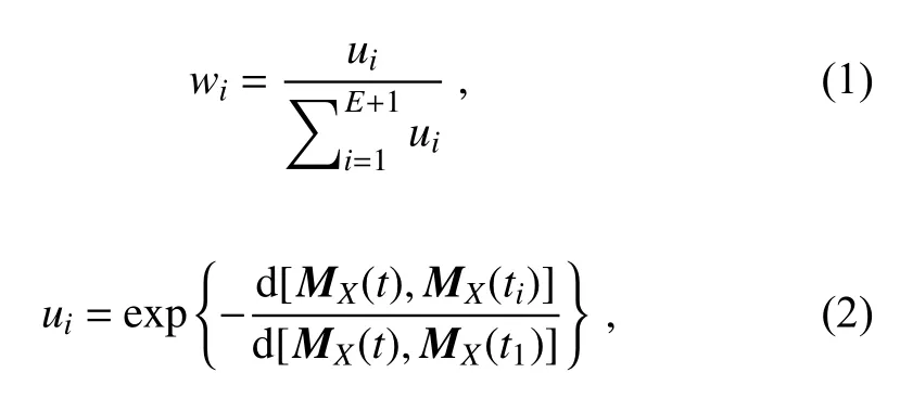
M
(t
),M
(t
)] denotes the Euler distance between vectorsM
(t
) andM
(t
). The most similar state to the timet
will occupy the largest weight.(iii) According to Tsonis et al. (2018),Y
at timet
can be estimated by


Y
toX
can also be measured referring to the above steps, labeled as ρ.ρrepresents how well the attractor ofX
can be used to reconstruct the time series ofY
, and if ρis of high magnitude, then it means that the information ofY
is encoded in the attractor ofX
through the causal influence fromY
toX
(Sugihara et al., 2012). Sugihara et al. (2012) and Tsonis et al. (2018) defined the causal inference from ρand ρas follows: (i) if ρis convergent whenL
is increased, and ρis statistically significant in the surrogate test, thenY
is suggested to be a causation ofX
. (ii) Moreover, if ρis also convergent whenL
is increased, and statistically significant in the surrogate test, then the causal relationship betweenX
andY
is bidirectional (X
andY
cause each other).CCM is an effective method for detecting the causality in a coupled nonlinear system; however, one should note that there are limitations, especially under the circumstance of strong coupling. As previously reported (Sugihara et al.,2012; McCracken and Weigel, 2014; Mønster et al., 2016,2017; Ma et al., 2018), the non-zero cross mapping skill may not reflect the real coupling direction in the presence of strong coupling or even intermediate coupling. Using CCM,it may not be easy to distinguish the real causality relations from the symmetric coupling. Furthermore, the existence of noise may also reduce the cross mapping skill. Therefore,the detected causality from the CCM needs to be considered with caution, and its time-lagged version, the timelagged CCM, is sometimes required.
2.2.2.2. Time-lagged CCM
Time-lagged CCM performs better in detecting causality relations in the presence of a strong coupling effect and random noise and can further estimate the delay effect of causal interaction, according to Ye et al. (2015). When detecting a causal influence fromY
(t
+t
) toX
(t
) (t
denotes the time lag and accepts both 0, positive and negative values) in a delayed-coupled system, it is assumed that the information ofY
(t
+t
) has been encoded toX
(t
), so that the value ofY
(t
+t
) can be reconstructed fromX
(t
) (Takens, 1981;Ye et al., 2015). Following the computation algorithm of the CCM, one can useX
(t
) to cross mapY
(t
+t
) with different values oft
, and estimate the cross mapping skill ρ(t
). Previous studies (Ye et al., 2015; Wang et al.,2018b) suggest that an optimal lag will exist where the cross mapping skill reaches its maximum. This optimal lag is determined by the delay time of the dynamical system(Ye et al., 2015), and we can use this optimal lag to identify the causality direction and the dynamical delay time between two coupled variables.As suggested in Ye et al. (2015), the causal relationship between two variables can be identified according to the following new criterion of causal inference: (i) if the maximum of ρ(t
) occurs at a negative lag (i.e.,t
< 0), this means that the information ofY
at the past time is encoded in the current state ofX.
In other words, the current state ofX
can be used to reconstructY
at the past time. In this case,Y
causesX
; (ii) if the maximum of ρ(t
) occurs at a positive lag, this means that the information ofY
at the future time is determined by the current state ofX.
In this case, the current state ofX
can be used to reconstructY
at the future time, andX
causesY
. Based on this new criterion, the timelagged CCM can produce robust results of the causality directions and avoid the weakness of the CCM. Therefore, compared with the causal inference of CCM (without time lag),this new causal inference from time-lagged CCM analysis has been found to be more accurate in the presence of a strong coupling effect and random noise (Ye et al., 2015;Huang et al., 2020); see also Figs. S1-S3 in the ESM. In this study, we apply the time-lagged CCM to study the causal relations between the AT and the ST at multiple layers.3. Effects of AT on the underlying ST of different layers
3.1. Impact strengths and time lags of the AT on the underlying ST
The AT variability can propagate downward to the deep soil layers (Beltrami and Kellman, 2003; Hu and Feng,2005; Chudinova et al., 2006), but the signal decays during the propagation, and the significance of the AT effects on the ST in deep layers is doubtful. Compared to the timelagged linear correlation analysis (Fig. S4 in the ESM),time-lagged CCM can distinguish the true causal relationship from the phenomenon of synchrony even if the variables are nonlinearly coupled (Sugihara et al., 2012; Ye et al., 2015; Wang et al., 2018b). Before the analysis of the causality from the AT to the STs, we first tested whether nonlinear processes were reflected in the time series of the variables of interest. As shown in Fig. S5 and Fig. S6 in the ESM, using simplex projection (Sugihara and May, 1990)the optimal embedding dimension (E
) was calculated. Then,using the S-map method (Sugihara, 1994) based on thisE
,we found the time series of both the AT and the STs have nonlinear signals, suggesting that nonlinear causal inference analysis (CCM or its time-lagged version) is necessary. Accordingly, based on the monthly anomaly time series (data length: 648 months), time-lagged CCM was thus employed to detect the strength (the maximum of the cross mapping skills for different time lags in time-lagged CCM) and the time lag of the impacts of the monthly AT on the ST at different layers. As shown in Fig. 1, the AT impacts on the ST are regionally different. With the increase in depth, the impact intensity decays rapidly, but the cross mapping skills of the CCM at all layers are statistically significant at the 99% confidence level (first column in Fig. 1). It takes time for the signals from the AT to propagate downward to the soil layers. At the depth of 40 cm, the responses of the ST to the AT variability at most stations are either “synchronous”or have one-month lags (right-hand column in Fig. 1). Only at several stations in northeastern China and northern Xinjiang province is the time taken to propagate downward to 40 cm longer than one month. It is worth noting that the detected “synchronization” is actually limited by the temporal resolution (i.e., monthly) of the data, as the time-lagged CCM cannot detect time lags shorter than one month. For more precise information, datasets with higher temporal resolution(e.g., daily) are required. With the depth increasing, the time lags increase from around one month at 40 cm to even ten months at some stations at 320 cm. Note that the AT and ST are weakly coupled in northeastern China. The cross mapping skills in this region are obviously smaller than in other regions. This may be a result of the fact that the influences of the AT take more time to propagate downward to the deep soil layers, and thus the intensity decays more.However, the mechanisms for this phenomenon are still unclear. It may be related to the soil type, but further studies are needed.3.2. Impacts of AT versus the impacts of soil memory from the previous season
Since the impacts of AT decay with the increase in depth, one may ask whether its impacts still dominate the variations of the ST at deeper layers. Particularly, in view of the strong soil memory in deep layers, is there a depth where the effects of soil memory become more important? To answer this question, the impact intensities of the AT and the soil memory on the ST in different seasons were compared in terms of the CCM coefficient ρ, whereY
represents the ST in the preceding seasons or the AT, whileX
represents the ST in the considered season. Note that, due to the data resolution (seasonal data, for example, spring series from 1960 to 2013) required in this analysis, we could not apply time-lagged CCM here. Instead, we employed CCM and only compare the AT effects of a considered season with the soil memory effects accumulated from one season before. Although the CCM coefficients may be affected by noise or the strength of the coupling, since the true causality from the AT to the STs (AT effects) has been detected by the time-lagged CCM (Fig. 1) and the pairwise asymmetric inference (PAI) method (Fig. S7 in the ESM) suggested by McCracken and Weigel (2014), to some extent the CCM coefficients may reflect the relative intensities of the AT effects versus the soil memory effects. Figure 2 shows that,in all seasons, the AT effects are always statistically significant at different layers, while the soil memory effects become consistently significant only from deep layers (≥160 cm) (right-hand column in Fig. 2). With the increase in depth, the AT effects decrease but the soil memory effects increase. At the depth of 160 cm, one can already see that effects of the soil memory can exceed those of the AT in summer (June-August), autumn (September-November) and winter (December-February). With further depth, i.e., at 320 cm, the soil memory effects eventually exceed the AT effects in all seasons and become more important. It is worth noting that the soil memory effects in northeastern China may be stronger, because when excluding the stations in northeastern China (left-hand column in Fig. 2),the soil memory effects become weaker. At the 160 cm layer, the soil memory effects are weaker than the AT effects (except for the effects in autumn), and only at the 320 cm layer are the soil memory effects significant in all seasons.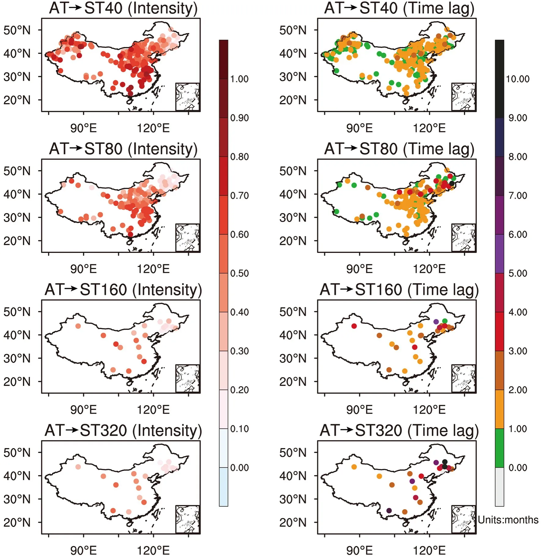
Fig. 1. Cross mapping skills of the CCM between the AT and the ST at different layers (ST40, ST80, ST160, ST320)(left-hand column) and the cross mapping lag for the response of the STs to the variations in the AT (right-hand column; units: months). Cross mapping skills of the CCM at all stations are statistically significant at the 99%confidence level.
4. Seasonal AT and ST trends during the recent global warming hiatus
4.1. Comparison of the AT and ST trends in different seasons
During the first decade of the 21st century there was a warming slowdown in the global mean surface temperature.When different seasons are considered, however, the hiatus did not occur everywhere. In the last section, significant AT impacts on the subsurface ST were found at all stations and all soil layers. Therefore, the ST trends are supposed to be similar to the AT trends, regardless of warming or cooling.As shown in Fig. S8 in the ESM, the spatial distribution of the AT and ST trends are similar in spring, summer and autumn. As for winter, however, the cooling trends of the AT in northeastern China have not been replicated by the STs in this region. On the contrary, continuous warming trends in the STs from 0 cm to 320 cm can be seen during the warming hiatus period (Fig. 3).
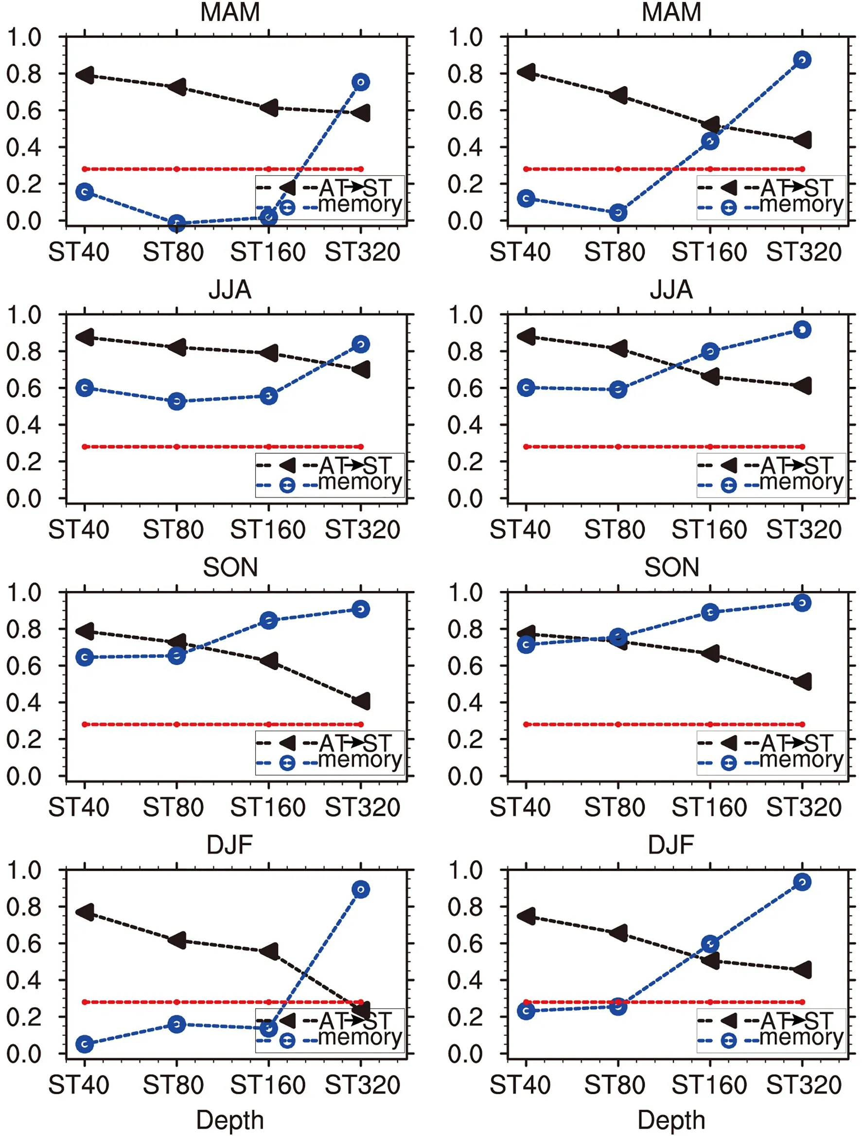
Fig. 2. Cross mapping skills of the CCM between the STs and (i) the AT (black dashed line) and (ii) the STs in the previous season (blue dashed line). The right-hand column shows the results with all stations included, while the lefthand column excludes the stations in northeastern China. Above the red dashed line indicates the greater than 95%confidence level. MAM, March-May; JJA, June-August; SON, September-October; DJF, December-February.
For a closer look of the trends, the third column of Fig. 3 shows the time series of the winter AT and winter ST at different depths averaged over northeastern China. It is clear that they all have similar trends from 1960, but since 1998, the trends between the AT and the ST display opposite signs(Fig. 3). A dramatic increase in ST0 is apparent from 1998 to 2013, and this is mainly attributable to the change in the observational infrastructure in 2005. Before 2005, the winter surface ST was usually measured manually on the bare ground. After the use of automatic measurement instruments in 2005, however, the ST0 was measured automatically even when the ground was snow covered. Thus, higher temperatures may be measured after 2005 (Xu et al., 2019).In spite of this, however, the ST0 still increases after 2005,and this warming cannot be explained by the change in the observational infrastructure. With increased depth, the ST trend becomes weaker. For the ST40, ST80, ST160 and ST320 layers, the linear trends from 1998 to 2013 are 0.544°C (10 yr), 0.472°C (10 yr), 0.071°C (10 yr)and 0.15°C (10 yr), respectively. To identify the start time of the warming trend, 15-year trends of the ST were calculated. It was found that the trends of ST40 and ST80 experienced a negative-to-positive change at the beginning of the 21st century, while those of ST160 and ST320 have been positive since the mid-1970s. This implies that the warming of the soil below 160 cm from 1998 to 2013 may be part of a persistent warming at a longer time scale. In other words, the physical processes related to the wintertime ST variability seem to vary with depth.
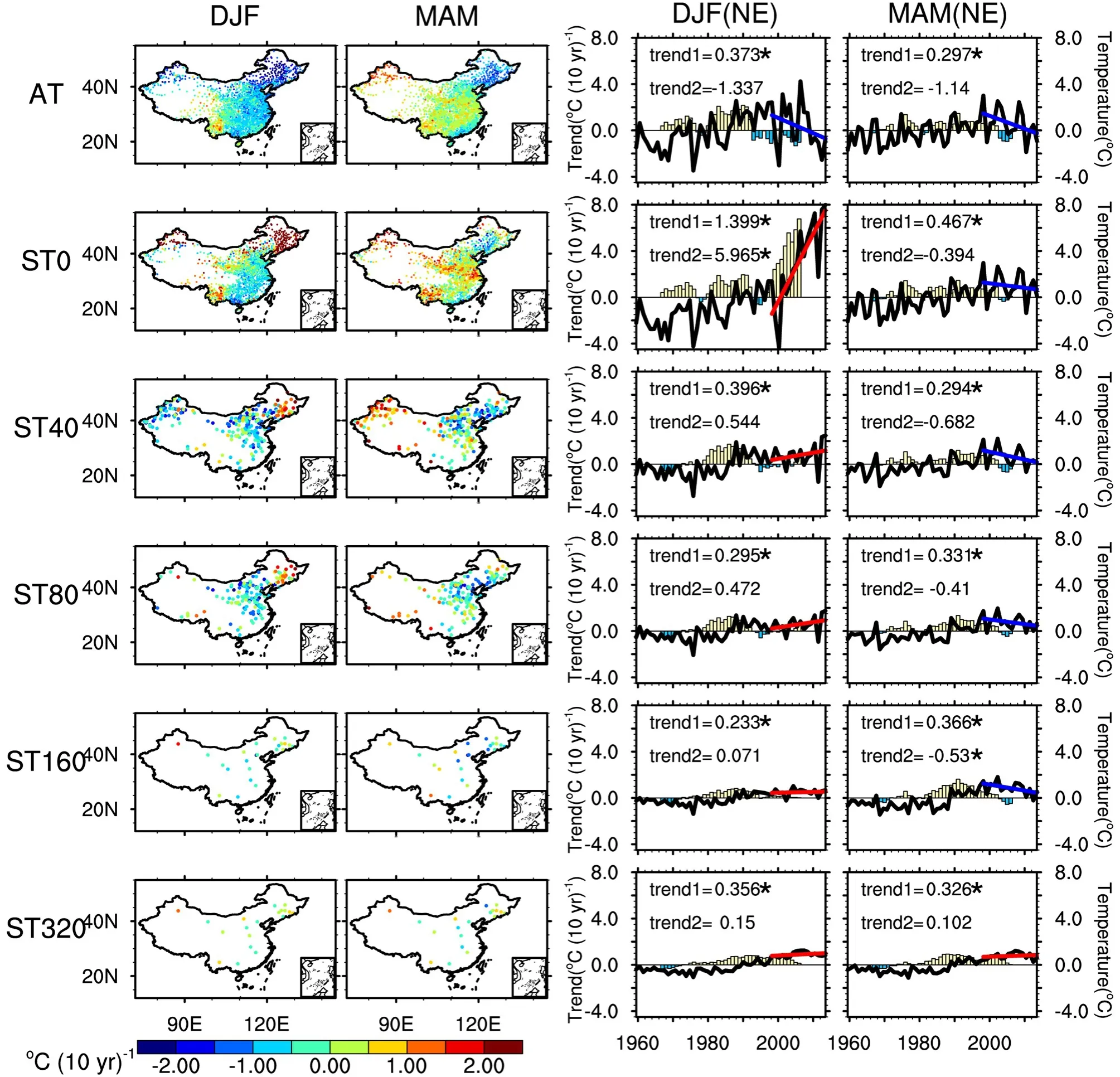
Fig. 3. Linear trends of the AT and STs (ST0, ST40, ST80, ST160, ST320) in winter (first column) and spring (second column) from 1998 to 2013. The spatial averages over northeastern China are shown in the third (winter) and fourth (spring) columns. “trend1”indicates the temperature changes from 1960 to 2013 and “trend2” shows the results from 1998 to 2013. “*” indicates the trends are statistically significant at the 95% confidence level. The curves are the time series of the anomalous AT and STs in northeastern China (right-hand vertical axis of the panels in the third and fourth columns; units: °C). The bars show the trends calculated from the sliding 15-year windows [left-hand vertical axis of panels in the third and fourth columns; units: °C (10 yr)-1].
When spring comes, the situation becomes completely different. The trend deviations between the AT and the ST almost disappear in northeastern China. Except for the ST at 320 cm, decreasing trends in ST are found at most stations in northeastern China, as well as in the spatial averages during the warming hiatus period (Fig. 3). The 15-year trends further reveal a positive-to-negative change at the beginning of the 21st century.
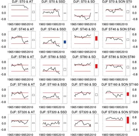
Fig. 4. The curves show the 15-year sliding correlation coefficients between the winter ST and four variables in northeastern China:the AT (first column), SSD (second column), SD (third column) and autumn ST (fourth column). Above the upper red line or below the bottom red line indicates the correlation coefficients are statistically significant at the 95% confidence level. The bars show the correlation coefficients from 1960 to 2013. The solid bars indicate the correlation coefficients are statistically significant at the 95%confidence level. All correlation coefficients were calculated after removing the trends of the time series.
4.2. Potential reasons for the soil warming
To understand the observed warming trend of the ST at different layers in winter, potential factors including the SD(the SD exceeds 4 cm in northeastern China, as shown in Fig. S9 in the ESM), the AT, the autumn ST, and the SSD were first studied using linear correlation analysis (Fig. 4).Considering the inhomogeneity of the ST0 (see previous section), in this section we only focus on the subsurface ST from 40 cm to 320 cm. The weak coupling between the AT and the ST in northeastern China was reconfirmed by the nonsignificant linear correlation coefficients (first column in Fig. 4). The SSD was found to be closely related with the ST40, but the correlation is negative, reflecting indirect relations between the SSD and the ST40. The effects of AT and SSD seem to be blocked by the effects of the snow cover, as significant positive correlations between the ST and the SD were found at the depths of 40 cm and 80 cm. The 15-year sliding correlations further indicate that the positive relations between the SD and the ST were stable in the past four decades and became more significant after the mid-1990s.This finding may be related to the insulation effect of the thicker snow cover. As reported in Zhang (2005), an increase in SD by 5 to 15 cm can lead to a 1°C increase in ground temperature. In the past few decades, large-scale wintertime cooling and increased snowfall over Eurasia have been found (Cohen et al., 2012; Tang et al., 2013; Luo et al., 2017). In this context, the SD in northeastern China has become thicker, and the spatial pattern of the SD increasing trend (Fig. S9) was found to be similar to the ST trends at the layers of 40 cm and 80 cm. Moreover, the 15-year trends of the SD in northeastern China also reveal a negative-to-positive change at the beginning of the 21st century(figure not shown). These facts support the inference that the thicker snow cover may contribute to the warmer ST at these two layers.
With the increase in depth, the correlations between the ST and the SD become nonsignificant, but the ST memory gradually starts to dominate. At the depth of 160 cm, the ST in autumn was found to be closely related to the ST in winter, but the 15-year sliding correlations reveal significant correlations only before 1980. For the ST at 320 cm, the memory from the previous season seems to have bigger impacts, as the correlation coefficients between the ST in autumn and the ST in winter are consistently significant over the past few decades. Accordingly, the memory effects from autumn may be important for the winter ST at deep layers. It is worth noting, however, that the persistent impact from autumn seems to mainly contribute to the interannual variations of the winter ST. It may not be possible to explain the slightly increasing trends of the winter ST at 160 cm and 320 cm by the memory effect from autumn, as the autumn ST at 160 cm and 320 cm does not exhibit increasing trends in northeastern China during the warming hiatus(Fig. S8).
Due to the time series of the SD (seasonal data) having nonlinear signals (Fig. S10 in the ESM), to further confirm the effects of the SD and the soil memory on the variations in ST at different layers, in the rest of this section the CCM method was applied (Fig. S11 in the ESM). In line with the results of linear correlation analysis (Fig. 4), the causal effects of the SD on the ST40 and ST80 in winter are remarkable, with the cross mapping skills nearly converging to 0.4 and 0.3, respectively. As for the ST at deeper layers,however, the cross mapping skills between the SD and the ST160 (ST320) almost vanish, indicating no causal effects.To rule out the potential biases induced by the drawbacks of the CCM (see Methods section), we further applied the PAI method (McCracken and Weigel, 2014) to check the causal relations detected by the CCM. As shown in Fig. S12 in the ESM, the causal effects of the SD on the winter ST at shallower layers (i.e., 40 cm and 80 cm) are confirmed well,without doubt. Regarding the effect of the soil memory on the winter ST, the CCM analysis indicates that the autumn ST has significant impacts on the winter ST at 320 cm, with the cross mapping skill nearly converging to 0.75. As for the ST at 160 cm, the CCM analysis does not infer a certain causality between the autumn ST and the winter ST, as the cross mapping skill is not convergent, indicating this depth might be a transition layer where the ST is influenced by the combined effects of both the snow cover and the soil memory.
5. Conclusions
In this study, responses of ST to different factors, including the surface AT, the snow cover, as well as the memory effects, were analyzed using ST data of different depths (0 cm to 320 cm) over China. Beyond previous studies that were mainly based on linear correlation analyses, this work investigated their relations using the CCM method and its time-lagged version, which can reveal the causality relations between the factors and the ST. As one of the most important factors, the AT was found to have significant impacts on the ST at all the considered depths, but the influence becomes weaker with the increase in depth. The memory effects, on the contrary, become more important with increased depth. At the depth of 320 cm, the thermal conditions from previous seasons were found to have stronger impacts than those from the AT of the considered season,indicating a possible change in the main controlling factor of the subsurface ST.
At shallower layers, the effects of AT on the ST are strong, but they may still be blocked by the change in land cover, e.g., the snow cover, in which case it is not easy for the signals from the AT to propagate downward into the soil and the corresponding effects are weakened. For instance,in northeastern China, the wintertime AT exhibited a decreasing trend during the recent global warming hiatus period,while the underlying ST showed an increasing trend. This unexpected increase was attributed to the increasing SD,which prevented the loss of heat from the soil to the atmosphere in winter. A detailed CCM analysis further revealed that the thermal insulation effect of the snow cover significantly affected the ST till the layer at 80 cm. It is worth noting that the snow cover in northeastern China becomes very thin in spring, and the thermal isolation effect very weak.The springtime ST showed a decreasing trend from 1998 to 2013, which was consistent with the AT.
These findings describe a physical picture of how the ST at different depths is influenced by different factors.They may be helpful for better understanding ST variabilities and land-atmosphere interactions. However, there are still some issues to be discussed. Firstly, limited by the observational ST dataset, we only focused here on stations in China. Whether the conclusions drawn in this study are applicable in other regions needs further study in the future.Secondly, one should note that the CCM analysis only revealed the causality relations from the AT to the ST. In the opposite direction, the influences of the ST on the AT were not detected. Recently, the mystery of the warming hiatus has been unpacked, and the heat redistribution processes in the oceans have been reported as a key reason.The fact that more energy is transferred and restored in the deep ocean is suggested as the main explanation for the slowdown in the warming trend. Similarly, did land-related processes also contribute to the warming hiatus? More specifically, since the ST has been considered as an important predictor for future climate change on seasonal time scales,does the ST affect the AT? And if so, how? To address these questions and further improve our understanding of land-atmosphere interactions, further research efforts in the future remain an urgent necessity.
. This work was sponsored by the National Key R&D Program of China (Grant No.2016YFA0600404) and the National Natural Science Foundation of China (Grant Nos. 41530532 and 41675088). N. Y. also thanks the support from the Chinese Academy of Sciences Pioneer Hundred Talents Program.Supplementary material is available in the online version of this article at https://doi.org/10.1007/s00376-020-0074-y.杂志排行
Advances in Atmospheric Sciences的其它文章
- A New Global Solar-induced Chlorophyll Fluorescence (SIF) Data Product from TanSat Measurements
- Phase Two of the Integrative Monsoon Frontal Rainfall Experiment (IMFRE-II) over the Middle and Lower Reaches of the Yangtze River in 2020
- Integrative Monsoon Frontal Rainfall Experiment (IMFRE-I):A Mid-Term Review
- Intermodel Diversity of Simulated Long-term Changes in the Austral Winter Southern Annular Mode: Role of the Southern Ocean Dipole
- Classification of Northeast China Cold Vortex Activity Paths in Early Summer Based on K-means Clustering and Their Climate Impact
- Determination of Surface Precipitation Type Based on the Data Fusion Approach
