How machine learning conquers the unitary limit
2021-04-12BastianKaspschakandUlfMeiner
Bastian Kaspschakand Ulf-G Meißner
1 Helmholtz-Institut für Strahlen- und Kernphysik and Bethe Center for Theoretical Physics,Universität Bonn,D-53115 Bonn,Germany
2 Institute for Advanced Simulation,Institut für Kernphysik,and Jülich Center for Hadron Physics,Forschungszentrum Jülich,D-52425 Jülich,Germany
3 Tbilisi State University,0186 Tbilisi,Georgia
Abstract Machine learning has become a premier tool in physics and other fields of science.It has been shown that the quantum mechanical scattering problem cannot only be solved with such techniques,but it was argued that the underlying neural network develops the Born series for shallow potentials.However,classical machine learning algorithms fail in the unitary limit of an infinite scattering length.The unitary limit plays an important role in our understanding of bound strongly interacting fermionic systems and can be realized in cold atom experiments.Here,we develop a formalism that explains the unitary limit in terms of what we define as unitary limit surfaces.This not only allows to investigate the unitary limit geometrically in potential space,but also provides a numerically simple approach towards unnaturally large scattering lengths with standard multilayer perceptrons.Its scope is therefore not limited to applications in nuclear and atomic physics,but includes all systems that exhibit an unnaturally large scale.
Keywords: unitary limit,machine learning,quantum physics
1.Introduction
After neural networks have already been successfully used in experimental applications,such as particle identification,see e.g.[1],much progress has been made in recent years by applying them to various fields of theoretical physics,such as[2,4,3,5–14].An interesting property of neural networks is that their prediction is achieved in terms of simple mathematical operations.A notable example is given by multilayer perceptrons (MLPs),see equation (4),that approximate continuously differentiable functions exclusively by matrix multiplications,additions and componentwise applied nonlinear functions.Therefore,a neural network approach bypasses the underlying mathematical framework of the respective theory and still provides satisfactory results.
Despite their excellent performance,a major drawback of many neural networks is their lack of interpretability,which is expressed by the term‘black boxes’.However,there are methods to restore interpretability.A premier example is given in[10]:by investigating patterns in the networks’weights,it is demonstrated that MLPs develop perturbation theory in terms of Born approximations to predict natural S-wave scattering lengths a0for shallow potentials.Nevertheless,this approach fails for deeper potentials,especially if they give rise to zero-energy bound states and thereby to the unitary limita0→∞.The physical reason for this is that the unitary limit is a highly non-perturbative scenario.In addition,the technical diffciulty of reproducing singularities with neural networks emerges,which requires unconventional architectures.Note that in its initial formulation,the Bertsch problem for the unitary Fermi gas includes a vanishing effective ranger0→0as an additional requirement for defniing the unitary limit,see e.g.[15].However,r0is non-zero and fniite,that is it violates scale invariance,fora0→∞in real physical systems,on which we want to focus in this work.Therefore,the casea0→∞we consider as the unitary limit,is independent of the effective range and,thus,less restrictive than the defniition in the Bertsch problem.The unitary limit plays an important role in our understanding of bound strongly interacting fermionic systems[16–21] and can be realized in cold atom experiments,see,e.g.[22].Therefore,the question arises how to deal with such a scenario in terms of machine learning? Our idea is explain the unitary limit as a movable singularity in potential space.This formalism introduces two geometric quantities f and b0that are regular fora0→∞and,therefore,can be easily approached by standard MLPs.Finally,natural and unnatural scattering lengths are predicted with suffciient accuracy by composing the respective networks.
The manuscript is organized as follows: in section 2,we introduce the concept of unitary limit surfaces and define a scale factor f,that allows to describe the potential around the first unitary limit surface.In section 3 we determine this factor with an ensemble of MLPs which is followed in section 4 with the determination of the scattering length a0in the vicinity of the first unitary limit surface.We pick up the issue of interpretability in section 5,using the Taylor expansion around a suitably chosen point on the first unitary surface.We end with further discussions and an outlook in section 6.Various technicalities are relegated to the appendices.
2.Discretized potentials and unitary limit surfaces
As we investigate the unitary limit,we only consider attractive potentials.For simplicity,the following analysis is restricted to non-positive,spherically symmetric potentials V(r)≤0 with finite range ρ.Together with the reduced mass μ,the latter parameterizes all dimensionless quantities.The most relevant for describing low-energy scattering processes turn out to be the dimensionless potential U=−2μρ2V≥0 and the S-wave scattering length a0.An important first step is to discretize potentials,since these can then be treated as vectorsU∈ Ω ⊂ Rdwith non-negative components Un=U(nρ/d)≥0 and become processable by common neural networks.We associate the piecewise constant step potential

where the rn=n/d for n=0,…,d andrd+1= ∞are the transition points of the given potential,with a real vectorU∈Ω.The components Unof this vector correspond to the individual values,the step potential in equation (1) takes between the(n −1)th and the nth transition point.In the following,we,therefore,refer to vectorsU∈Ωas discretized potentials.The degree d of discretization thereby controls the granularity and corresponds to the inverse step size of the emerging discretized potentials.Choosing it sufficiently large ensures that the entailed
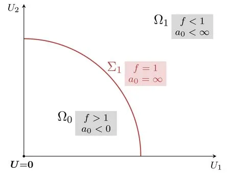
Figure 1.Sketch of the regions Ω0 and Ω1 and the first unitary limit surface Σ1 ⊂Ω1 for the degree d=2 of discretization.In this specific case,the potential space Ω is the first quadrant ofR2 and unitary limit surfaces are one-dimensional manifolds.discretization error,e.g.on the scattering length,becomes insignificantly small.For instance,taking d=64 as in the following analysis reproduces the basic characteristics of all considered potentials and satisfies that requirement.
As a further result of discretization,the potential space is reduced to the first hyperoctant Ω ofRd.Counting bound states naturally splits Ω=⋃i∈N0Ωiinto pairwise disjunct,half-open regions Ωi,with Ωicontaining all potentials with exactly i bound states.All potentials on the d−1 dimensional hypersurfacebetween two neighboring regions with Σi⊂Ωigive rise to a zero-energy bound state,see figure 1.Since we observe the unitary limita0→∞in this scenario,we refer to Σias the ith unitary limit surface.Considering the scattering length as a functiona0: Ω →R,this suggests a movable singularity on each unitary limit surface.For simplicity,we decide to focus on the first unitary limit surface Σ1,as this approach easily generalizes to higher order surfaces.LetU∈Ωandf∈+R be a factor satisfyingfU∈Σ1.This means scalingUby the unique factor f yields a potential on the first unitary limit surface.While potentials with an empty spectrum must be deepened to obtain a zero-energy bound state,potentials whose spectrum already contains a dimer with finite binding energy E<0 need to be flattened instead.Accordingly,this behavior is reflected in the following inequalities:

3.Predicting f with an ensemble of MLPs
The factor f seems to be a powerful quantity for describing the geometry of the unitary limit surface Σ1.The latter is merely the contour for f=1.It is a simple task to derive f iteratively by scaling a given potentialUuntil the scattering length flips sign,see appendix A.However,an analytic relation betweenUand f remains unknown to us.The remedy for this are neural networks that are trained supervisedly on pairs(U,f) ∈T1of potentials(inputs) and corresponding factors (targets) in some training set T1.In this case,neural networks can be understood as maps F: Ω →Rthat additionally depend on numerous internal parameters.The key idea of supervised training is to adapt the internal parameters iteratively such that the outputs F(U)approach the targets f ever closer.As a result of training,F approximates the underlying functionU↦f,such that the factorf* ≈F(U*) is predicted with sufficient accuracy even if the potentialU*∈Ωdoes not appear in T1,as long as it resembles the potentials encountered during training.This is also referred to as generalization.In order to measure the performance ofF on unknown data,one considers a test set T2containing new pairs(U*,f*) and the mean average percentage error (MAPE) on that set,

By generating randomized inputsUvia Gaussian random walks,we ensure that the training set covers a wide range of different potential shapes,see appendix A.This is extremely important,since we want to avoid the neural network to overfit to specific potential shapes and instead to optimally generalize over the given region of interest around Σ1in potential space.
We decide to work with MLPs.These are a widely distributed and very common class of neural networks and provide an excellent performance for simpler problems.Here,an MLPFiwith L layers is a composition

of functionsY j:Vj−1→Vj.Usually we haveVj= Rhj.WhileY1: Ω →V1andYL:VL−1→R are called the input and output layers,respectively,each intermediate layer is referred to as a hidden layer.The layer Yjdepends on a weight matrixand a biasboth serving as internal parameters,and performs the operation

on the vectorv∈Vj−1.The functionaj: R→R is called the activation function of the jth layer and is applied componentwise to vectors.Using nonlinear activation functions is crucial in order to make MLPs universal approximators.While output layers are classically activated via the identity,we activate all other layers via the continuously differentiable exponential linear unit (CELU) [23],

We use CELU because it is continuously differentiable,has bounded derivatives,allows positive and negative activations and finally bypasses the vanishing-gradient-problem,which renders it very useful for deeper architectures.In order to achieve precise predictions of the factors f,we decide to train an ensemble ofFN=100 MLPsFi,with each MLP consisting of nine CELU-activated 64×64 linear layers and one output layer.Thereby,an ensemble can be understood as a point cloud in weight space with the ith point representingFi.We choose the output of the ensemble to be simply the mean of all individual outputs,
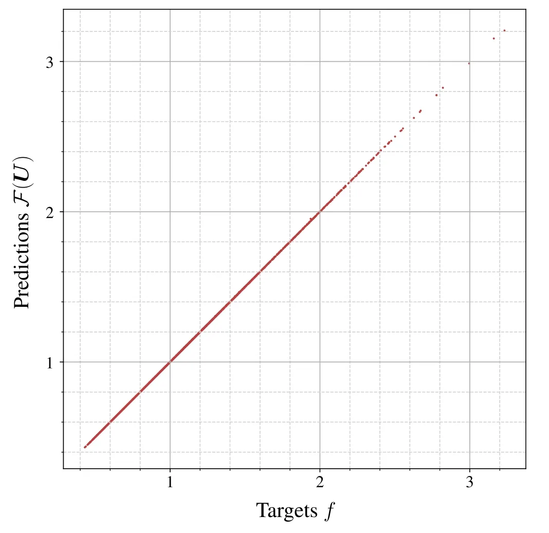
Figure 2.Predictions F (U) of the scaling factor by the ensemble F versus the targets f for all(U ,f) ∈T2.The resulting point cloud is very closely distributed around the bisector,which indicates an excellent performance ofF on the test set T2.

The training and test data sets contain∣T∣1=3×10⁴and∣T∣2=2.9×10³samples,respectively,with the degree d=64 of discretization,as described in appendix A.Positive and negative scattering lengths are nearly equally represented in each data set.After 20 epochs,that is after having scanned through the training set for the 20th time,the training procedure is terminated and the resulting MAPE of the ensembleF turns out as 0.028%.When plotting predictions versus targets,this implies a thin point cloud that is closely distributed around the bisector as can be seen in figure 2.We therefore conclude that F returns very precise predictions on f.
4.Predicting scattering lengths in vicinity of Σ1
Our key motivation is to predict scattering lengths in vicinity of Σ1.Being a movable singularity in potential space,the unitary limit itself imposes severe restrictions on MLP architectures and renders training steps unstable.Therefore,we opt for the alternative approach of expressing scattering lengths in terms of regular quantities,that each can be easily predicted by MLPs.Given the factors f we first consider

Note thatx= (1 −f)‖U‖is the distance between the given potentialU∈ΩandfU∈Σ1.ForU∈Ω0,we observe x<0,whereas x=0 forU∈Σ1and x>0 else.The quantity b0provides an equivalent understanding of this distance in terms ofx=which does not explicitly depend on the factor f.
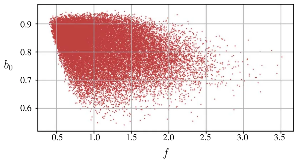
Figure 3.b0 versus the corresponding factors f for all potentials U in the training set T1.Note that b0 is restricted to a small interval.The width of the point cloud suggests that there is no one-to-one relation between b0 and f.
As shown in figure 3,b0is finite and restricted to a small interval for all considered potentials.This does not imply that f and b0are globally regular.Indeed,f diverges forU→0 and b0diverges on each higher order unitary limit surface.However,these two scenarios have no impact on our actual analysis.
Similar to the ensembleF in equation (7),we train an ensembleB ofNB=100 MLPs Bi.While the members Bionly consist of five CELU-activated 64×64 linear layers and one output layer,the rest coincides with the training procedure as presented in the previous section.The resulting MAPE ofB turns out as 0.017%.Since all potentials in T1are distributed around Σ1,this correspondingly indicates thatB approximates the relationU↦b0very well in vicinity of the first unitary limit surface.
Having trained the ensemblesB andF to predict b0and f precisely (see appendix B for details),we are able to construct scattering lengths according to equation (8): we expect the quotient

to provide a good approximation of a0for potentials in vicinity of Σ1.This may appear counterintuitive at first,since the scattering length has a clear physics interpretation,whereas the quantities b0and f refer to points and distances in potential space,that are not observable themselves.However,requiring all potentials to be of finite range suffices for a unique effective range expansion and thus renders this approach model-independent.Figure 4(a)shows scattering lengths for potential wells that are predicted byA.As expected,we observe a singularity for the depth u=π2/4.In the same figure,this is compared to the case,in which another ensembleA of ten MLPs Aiis given.These do not compute f and b0as intermediate steps,but have been trained to predict a0directly.However,since the Aiare continuously differentiable,a singularity cannot be reproduced.This retrospectively justifies the proposed approach in equation (9).
Note that outputs A(U) for potentials in the unitary limit f →1 are very sensitive to F(U) .In this regime,even the smallest errors may cause a large deviation from the target values and thereby corrupt the accuracy ofA.In figure 4(b) we observe significantly larger relative errorsεA(U)=(A(U) − a0)/a0in a small interval around the unitary limit at u=π2/4.Of course,this problem could be mitigated by a more accurate prediction of f,but the underlying difficulty is probably less machine-learningrelated and is rather caused by working with large numbers.Nonetheless,the quotientA reproduces the basic behavior of a0sufficiently well for our purposes.Inspecting the prediction-versus-target plot for the test set T2is another and more general,shape-independent way to convince ourselves of this,see figure 5.Although we notice a broadening of the point cloud for unnaturally large scattering lengths,the point cloud itself remains clearly distributed around the bisector.This implies thatA predicts natural and unnatural scattering lengths precisely enough and agrees with its low relatively low MAPE.Finally,the resulting MAPE of 0.41%indicates an overall good performance ofA on the test set T2.
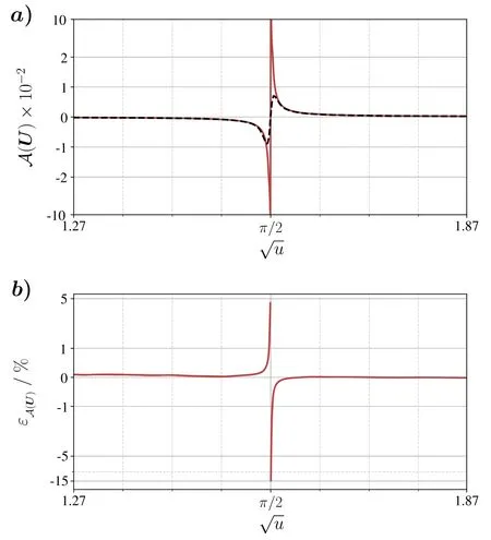
Figure 4.(a): Predicted scattering lengths A (U) for potential wells with depths u withA as given in equation (9) (solid red line) and,respectively,with an ensembleA of ten MLPs Ai that are trained to directly predict a0 (dashed black line).(b): Relative errorsεA( U) of predicted scattering lengths A (U) for potential wells with depths u.Theonly take values between 1%and 15%in close vicinity of the unitary limit and become negligibly small elsewhere.
5.Taylor expansion for interpretability
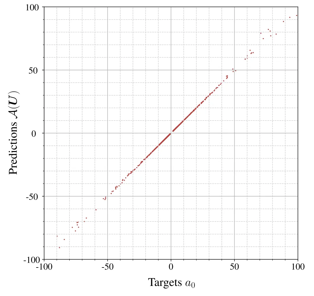
Figure 5.Predictions A (U) of scattering lengths by the quotientA versus the targets a0.The point cloud becomes broader for unnaturally large scattering lengths.Nonetheless it is still distributed sufficiently close around the bisector,which indicates thatA generalizes well and reproduces the correct behavior of a0 around Σ1.

with the displacementδU=U−U* and the vectornwith the componentsFor small displacements‖δU‖ ≪1 higher order terms in equation (10) become negligible.From construction we know that F(U*) ≈1for anyNote thatnis the normal vector of the first unitary limit surface at the pointU*.This is because F(U) is invariant under infinitesimal,orthogonal displacementsδU⊥n.
To give an example,we consider the first order Taylor approximation with respect to the potential wellin Σ1.At first we derive F(U* )=(1–3.19)×10−5.Due to the rather involved architecture of F,we decide to calculate derivatives numerically,that iswith the ith basis vectoreiand the step size Δ=0.01.In figure 6 we can see thatnis far from collinear toU*,which implies a complicated topology for Σ1.Using the expansion in equation(10)and the components nishown in figure 6,we arrive at an interesting and interpretable approximation of A(U) aroundU*,

Equation(11)allows us to interpret the unitary limit locally in terms of a scalar product,which reproduces the tangent plane of Σ1at the pointU* ∈Σ1.Successively inserting higher order terms of the Taylor series in equation (10) would correspondingly introduce curvature terms.Let us consider displacementsthat are parallel toU*,such thatU*+δUis a potential well with depth u.By insertingandequation (11)becomes
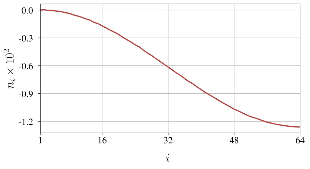
Figure 6.Components of the normal vector n of the unitary limit surface at .As a gradient ofF,this vector points towards the strongest ascent of f,which explains why its components are negative.

We can compare this to the expected behaviora0= 1 −tanof the S-wave scattering length for potential wells.The Padé-approximant of order [0/1] of this function at u=π2/4 is given bywhich agrees with the approximation equation (12) of scattering length predictions for inputsU=u(1 ,… ,1) in the vicinity ofU* by the quotientA.Using both approximations for A(U)and a0we obtain

as an estimate on the relative error.We convince ourselves that,up to a steep divergence for the depth u=π2/(4–7.92)×10−5due to a minor deviation in the root of the denominator,the relative errorεA(U)enters the per mille range,as we have already seen in figure 4(b).
6.Discussion and outlook
The unitary limita0→∞is realized by movable singularities in potential space Ω,each corresponding to a hypersurface Σi⊂Ωthat we refer to as the ith unitary limit surface.This formalism not only lets one understand the unitary limit in a geometric manner,but also introduces new quantities f and b0,that are related to the radial distance between the corresponding potentialUand the first unitary limit surface Σ1.These are regular in the unitary limit and provide an alternative parameterization of low-energy scattering processes.As such,they suffice to derive the S-wave scattering length a0.By training ensembles of MLPs in order to predict f and b0,respectively,we therefore successfully establish a machine learning based description for unnatural as well as natural scattering lengths.
There is one major problem that remains unresolved by the presented approach:predictions A(U) of unnaturally large scattering lengths sensitively depend on the precision of the ensembleF.Minor errors in f cause the predicted first unitary limit surface to slightly deviate from the actual surface Σ1.In very close neighborhood of the unitary limit,this generates diverging relative errors with respect to the true scattering lengths a0.As the predictions ofF will always be erroneous to a certain degree,this problem cannot be solved by optimizing the architecture or the training method.Instead,it is less machine-learning-related and rather originates in the handling of large numbers.However,the presented method involving f and b0is still superior to more conventional and naive approaches like predicting the inverse scattering length 1/a0,which is obviously regular in the unitary limit,and considering the inverse prediction afterwards.Although the latter would provide a good estimate on unnatural scattering lengths,too,it would fail for a0≈ 0,whereas the divergence of f for extremely shallow potentialsU∈Ω(that is‖U‖ ≪1)can be easily factored out usingfU=αfα·Ufor anysuch thatfα·Uis regular.For example,when choosingthe factorscorrespond to the radial coordinate of Σ1in the directionfrom the origin of Ω,which is clearly finite.Apart from the geometric interpretation of the unitary limit,which simply cannot be provided by classical approaches,we,therefore,conjecture the proposed method to offer the opportunity of simultaneously determining extremely large and small scattering lengths with sufficient precision.Nevertheless,it does not substitute a direct solution of the Schrödinger equation.The asymptotics of its solutions are required in order to compute the effective range function and,finally,the scattering lengths.As targets,the latter are an important part of supervised learning and have to be determined before initiating the training procedure.
We recall that both ensembles leave training as ‘black boxes’.By considering their Taylor approximations,we can obtain an interpretable expression of the predicted scattering lengths A(U) in terms of a scalar product.This also provides additional geometric insights like normal vectors on the unitary limit surface.
Note that the presented approach is far more general,than the above analysis of Σ1suggests and,in fact,is a viable option whenever movable singularities come into play.First of all,we could have defined the quantities f and b0with respect to any higher order unitary limit surface Σiwith i>1,since we can apply the same geometric considerations as for Σ1.Adapting the training and test sets,such that all potentials are distributed around Σiwould allow to trainF andB to predict f and b0,respectively,which finally yields scattering lengths in vicinity of Σi.This procedure is,however,not even limited to the description of scattering lengths and can be generalized to arbitrary effective range parameters,since these give rise to movable singularities,as well.To give an example,we briefly consider the effective range r0,which diverges at the zero-crossing of a0.In analogy to the unitary limit surfaces Σi,we could,therefore,define the ith zerocrossing surface Σi′as the d−1 dimensional manifold in Ωi,that contains all potentials with i bound states and a vanishing scattering lengtha0→0,such that∣r0∣ →∞.Here,we could define f′by scaling potentials onto a particular surface,that isfor allU∈Ω,and subsequentlyFrom this point,all further steps should be clear.Even beyond unitary limit and zero-crossing surfaces,analyzing how the effective range behaves under the presented scaling operation and interpreting the outputs of the corresponding neural networks seems to be an interesting further step from here in order to investigate effective range effects and deviations from exact scale invariance.
A downside of the presented method is that it is,as defined above,only capable of approaching one movable singularity Σi.In the case of scattering lengths,this is because b0diverges at each other unitary limit surfacewithi′ ≠idue to the divergence of a0and.Let us defineas the subset of all potentialsU∈Ωthat are surrounded by the above mentioned zero-crossing surfacesandthat is for allthere are α<1 and β≥1,such thatandThe problem can be solved by redefining f to scale potentials between two zero-crossing surfaces onto the enclosed unitary limit surface Σi+1,that isfU∈Σi+1for all∈UAs a consequence,f becomes discontinuous and behaves similar to an inverted sawtooth function,which accordingly requires to involve discontinuous activations in the MLPsFi.Note that even after the redefinition,b0remains continuous as it vanishes on the zero-crossing surfaces due to a0=0,which is exactly where the redefined f has a jump discontinuity.
The idea to study manifolds in potential space does not need to be restricted to movable singularities of effective range parameters,but can be generalized to arbitrary contours of low-energy variables.To give an example,consider the d−1 dimensional hypersurfacethat consists of all discretized potentialsU∈Ωthat give rise to i bound states and whose shallowest bound state has the binding energy B.Note that for B=0,this exactly reproduces the ith unitary limit surfaceIn this case,the shallowest bound state in a zero-energy bound state.Otherwise,that is ifB≠ 0,the scattering lengths of all points onmust be finite and,thus,there cannot be an overlap betweenand any unitary limit surface Σj,such that∩Σj= ∅for alli,j∈N.Here,unitary limit surfaces mark important boundaries between scattering states and bound state spectra:by crossing a unitary limit surface,a scattering state undergoes dramatic changes to join the spectrum as a new,shallowest bound state.When analyzing a given system in a finite periodic box,instead,zero-energy bound states resemble deeper bound states much more.In this context we refer to Lattice Monte Carlo simulations probing the unitary limit in a finite volume,see [24].
Acknowledgments
We thank Hans-Werner Hammer and Bernard Metsch for useful comments.We acknowledge partial financial support from the Deutsche Forschungsgemeinschaft (Project-ID 196253076 - TRR 110,‘Symmetries and the Emergence of Structure in QCD’),Further support was provided by the Chinese Academy of Sciences (CAS) President’s International Fellowship Initiative (PIFI) (Grant No.2018DM0034),by EU (Strong2020) and by Volkswagen-Stiftung (Grant No.93562).
Appendix A.Preparation of data sets
As a consequence of discretization,the lth partial wave is defined piecewise:between the transition points rn−1and rnit is given as a linear combination of spherical Bessel and Neumann functions,

with the kinetic energy

Here we introduce the factor

to conserve the sign of k on the complex plane,that iskn→k,if Unvanishes.The parametersAl,d+1(k)andBl,d+1(k)completely determine the effective range functionKl(k) =k2l+1cotδl(k)due to their asymptotic behavior

Instead of solving the Schrödinger equation for the step potential U(r),we apply the transfer matrix method [25] to deriveAl,d+1(k)andBl,d+1(k).Due to the smoothness of the partial waveφ(l,k)at each transition point rn,this method allows us to relateAl,d+1(k)andBl,d+1(k)to the initial parametersAl,1(k)andBl,1(k)via a product of transfer matricesMl,n(k).To arrive at a representation of these transfer matrices,we split up the mentioned smoothness condition into two separate conditions for continuity,

and differentiability,

at each transition point rn.Using equation (A1),we can combine both conditions (A6) and (A7) to a vector equation,that connects neighboring coefficients with each other:
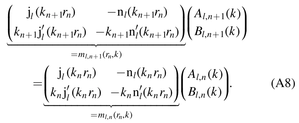
Multiplying equation (A8) withfrom the left yields

which defines the nth transfer matrix

Therefore,Al,d+1(k)andBl,d+1(k)are determined by the choice ofAl,1(k)andBl,1(k),which requires us to define two boundary conditions.Due to the singularity of nlin the origin,the spherical Neumann contribution in the first layer must vanish and thereforeBl,1(k) =0.The choice ofAl,1(k)may alter the normalization of the wave function.However,since we only consider ratios ofAl,d+1(k)andBl,d+1(k),we may opt forAl,1(k) =1,which corresponds to

Finally,applying all transfer matrices successively to the initial parameters yields

The most general way to derive any effective range expansion parameterfor arbitrary expansion points∈C in the complex momentum plane is a contour integration along a circular contour γ with radius κγaroundApplying Cauchy’s integral theorem then yields

We approximate this integral numerically over N grid points

Smaller contour radii κγand larger N thereby produce finer grids and decrease the approximation error.This way of calculatingrequiresin totald×N transfer matrices.The numerical integration provides

Despite the generality of equation (A15),we restrict this analysis to S-wave scattering lengthssince these dominate low-energy scattering processes.
While generating the training and test sets,we must ensure that there are no overrepresented potential shapes among the respective data set.To maintain complexity,this suggests generating potentials with randomized components Un.An intuitive approach therefore is to produce them via Gaussian random walks:given d normally distributed random variables X1,…,Xd,

where N (μ,σ)describes a normal distribution with mean μ and standard deviation σ,the distribution of the nth potential step Uncan be described by the magnitude of the sum over all previous steps Xi,

Figure A1.(a): Distribution of the square root of the average depth over the training set.By construction,this distribution is uniform.(b): Bimodal distribution of the scattering length a0 over the training set.Note that extremely large scattering lengths are not displayed in this histogram.

Note that,while all steps Xiin equation (A16) have zero mean,the standard deviation of the first step,which we denote by the initial step factor ISF,may differ from the standard deviation of all other steps,that we refer to as the step factor SF.This allows us to roughly control the shapes and depths of all potentials in the data set.Choosing ISF ≫ SF results more likely in potentials that resemble a potential well and expectedly yield similar scattering lengths.In contrast to that,SF ≫ ISF produces strongly oscillating potentials.We decide to choose the middle course ISF=1 and SF=0.75(this is the case SF ≈ISF)for two reasons:for one,from the perspective of depths,the corresponding Gaussian random walk is capable of generating potentials around the first unitary limit surface Σ1.For another,this choice of step factors causes the data set to cover a wide range of shapes from dominantly potential wells to more oscillatory potentials,which is an important requirement for generalization.This way,we generate 105potentials for the training set and 104potentials for the test set,To avoid overfitting to a certain potential depth,this needs to be followed by a rigorous downsampling procedure.For this,we use the average depth

as a measure.Uniformizing the training and test set with respect toon the interval [1.10,1.87] by randomly omitting potentials with overrepresented depths finally yields a training set T1,see figure A1,and test set T2that contain 3×10⁴and 2.9×10³potentials,respectively.Scattering lengths are then derived using the numerical contour integration in equation (A15) with N=100 grid points and a contour radius of κγ=0.1.The derivation of the factors f is more involved: if the scattering length is negative (positive),the potential is iteratively scaled with the factor s=2(s=1/2),until its scattering length changes its sign.Let us assume the potential has been scaled t times this way.Then we can specify the interval where we expect to find f in as(2t−1,2t]or as [2−t,21−t),respectively.Cubically interpolating 1/a0on that interval using 25 equidistant values and searching for its zero finally yields the desired factor f.
Appendix B.Training by gradient descent
Given a data setD⊆Ω × Rn,there are several ways to measure the performance of a neural networkN: Ω →Rnon D.For this we have already introduced the MAPE that we have derived for the test set D=T2after training.Lower MAPEs are thereby associated with better performances.Such a function Γ →+RL: that maps a neural network to a non-negative,real number is called a loss function.The weight space Γ is the configuration space of the used neural network architecture and as such it is spanned by all internal parameters (e.g.all weights and biases of an MLP).Therefore,we can understand all neural networksN∈Γof the given architecture as points in weight space.The goal all training algorithms have in common is to find the global minimum of a given loss function in weight space.It is important to note that loss functions become highly nonconvex for larger data sets and deeper and more sophisticated architectures.As a consequence,training usually reduces to finding a well performing local minimum.
A prominent family of training algorithms are gradient descent techniques.These are iterative with each iteration corresponding to a step the network takes in weight space.The direction of the steepest loss descent at the current position N∈Γ is given by the negative gradient ofL(t,N(U)).Updating internal parameters along this direction is the name-giving feature of gradient descent techniques.This suggests the update rule

for each internal parameter p,and by the left arrowa←bwe denote the assignment ‘a=b’ as used in computer programming.Accordingly,the entire training procedure corresponds to a path in weight space.The granularity of that path is controlled by the learning rate η: smaller learning rates cause a smoother path but a slower approach towards local minima and vice versa.In any case,training only for one epoch,that is scanning only once through the training set,usually does not suffice to arrive near any satisfactory minima.A typical training procedure consists of several epochs.
Usually,the order of training samples(U,t) is randomized to achieve a faster learning progress and to make training more robust to badly performing local minima.Therefore,this technique is also called stochastic gradient descent.Important alternatives to mention are mini-batch gradient descent and batch gradient descent,where update steps are not taken with respect to the lossL(t,N(U))of a single sample,but to the batch loss of randomly selected subsets D of the training set T1with the batch size∣D∣=Bor the entire training set itself,respectively.There are more advanced gradient descent techniques like Adam and Adamax [26] that introduce a dependence on previous updates and adapted learning rates.It is particularly recommended to use these techniques when dealing with large amounts of data and high-dimensional weight spaces.

For training the membersFiandBiof both ensemblesF andB,we apply the same training procedure using the machine learning framework provided by PyTorch [28]:weights and biases are initialized via the He-initialization[27].We use the Adamax optimizer with the batch size B=10 to minimize the L1-Loss,

over 20 epochs.Here,we apply an exponentially decaying learning rate scheduleIn this case,the decreasing learning rates allow a much closer and more stable approach towards local minima.
杂志排行
Communications in Theoretical Physics的其它文章
- First-principles study on superconductive properties of compressive strain-engineered cryogenic superconducting heavy metal lead (Pb)
- Majorana–Kondo interplay in a Majorana wire-quantum dot system with ferromagnetic contacts*
- Effect of Zn doping on electronic structure and optical properties zincblende GaN (A DFT+U insight)
- Exploring the influence of microRNA miR-34 on p53 dynamics: a numerical study*
- A new approach for modelling the damped Helmholtz oscillator: applications to plasma physics and electronic circuits
- Coexistence and fluctuations phenomena with Davidson-like potentials in quadrupole–octupole deformed nuclei
