Solving Severely Ill-Posed Linear Systems with Time Discretization Based Iterative Regularization Methods

，

College of Science，Nanjing University of Aeronautics and Astronautics，Nanjing 211106，P.R.China

（Received 11 March 2020；revised 29 April 2020；accepted 9 October 2020）

Abstract:Recently，inverse problems have attracted more and more attention in computational mathematics and become increasingly important in engineering applications.After the discretization，many of inverse problems are reduced to linear systems.Due to the typical ill-posedness of inverse problems，the reduced linear systems are often illposed，especially when their scales are large.This brings great computational difficulty.Particularly，a small perturbation in the right side of an ill-posed linear system may cause a dramatical change in the solution.Therefore，regularization methods should be adopted for stable solutions.In this paper，a new class of accelerated iterative regularization methods is applied to solve this kind of large-scale ill-posed linear systems.An iterative scheme becomes a regularization method only when the iteration is early terminated.And a Morozov’s discrepancy principle is applied for the stop criterion.Compared with the conventional Landweber iteration，the new methods have acceleration effect，and can be compared to the well-known accelerated ν-method and Nesterov method.From the numerical results，it is observed that using appropriate discretization schemes，the proposed methods even have better behavior when comparing with ν-method and Nesterov method.

Key words：linear system；ill-posedness；large-scale；iterative regularization methods；acceleration

0 Introduction

During the past fifty years，inverse problems have attracted more and more attention and have extensive applications in engineering and mathematical fields，such as Cauchy problem［1-3］，geophysical exploration［4］，steady heat conduction problems［5-6］，inverse scattering problems［7-9］， image processing［10-11］， and reconstructon of radiated noise source［12］etc.After the discretization，many of them are reduced to the ill-posed linear system as

Here by the ill-posed linear system，it means that the condition number of the coefficient matrixA∈Rm×nis much larger compared with the square of the scale ofA.Denote by the quasi-solution of Eq.（1）.There are three cases forx†：（i）The system admits a unique solution，thenx†is the exact solution；（ii） the system has more than one solution，thenx†is the one of minimal 2-norm among all solutions；（iii）the system has no solution，thenx†is least squares solution.It is easy to verify thatx†is unique.

Practically，boften comes from measurements or discretization，and contains inevitably noise.Instead ofb，assume we only have noisy databδat hand，satisfying

whereδis the noisy level and‖‖·the standard Euclidean norm of a vector.Therefore，in this paper we are devoted to find an approximate solution to the polluted linear system

Similarly，denote byxδthe unique quasi-solu-tion corresponding to the noisy databδ.

For an ill-posed system，a small disturbance inbwill lead to much large change in solutionx.This brings quite large difficulty when one solves the system numerically，especially when the scale is large.Thus，it is useless to use the conventional numerical methods to solve system（1）or（3）.In fact，by using the singular value decomposition（SVD），the solutions of Eq.（1）or（3）can be written formally as［13］

where{(σi，ui，vi)}are the singular values and singular vectors of the coefficient matrixA，satisfyingσ1≥σ2≥ …≥σr＞ 0，σi≤ 1fori≥kand some indexk≤r，ris the rank ofA.Therefore‖ ‖xδ-x†may be quite big even if‖ ‖bδ-bis small，and regularization methods are needed for obtaining a stable approximate solution toxδand thus also tox†.

Generally speaking，there are three groups of regularization methods：truncated singular value decomposition （TSVD）［13-15］， variational regularization methods［16-17］and iterative regularization methods［18-21］.For large-scale ill-posed problems，TSVD leads to computational difficulty in that the vast storage and the heavy computing burden.The most famous variational regularization method is Tikhonov’s regularization method［22］.Recently， a projection fractional Tikhonov regularization method is proposed［23］.However，during the determination of the regularization parameters，a forward problem has to be solved for each regularization parameter，which makes the calculation very large.Iterative regularization methods have the advantages of low computational cost and simple forms.Thus for large-scale problem，we prefer to use iterative regularization methods，where iterative schemes are proposed to solve the following optimization problem.

The most classic iterative regularization method should be Landweber iteration［24-25］.For the linear system（3），Landweber iteration is defined by

Eq.（5） can be viewed as a discrete analog of the following first order evolution equation.

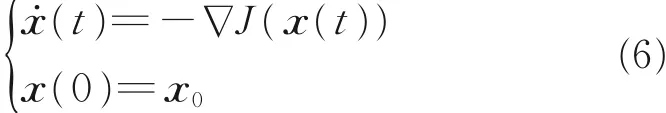
wheretis the introduced artificial time，andx0an initial guess tox†.The formulation（6）is known as an asymptotical regularization，or the Showalter’s method［26-27］.It is well known that the Landweber method converges quite slowly［28］.Thus，it is no wonder that accelerating strategies are adopted in practice.In recent years，there has been increasing evidence to show that the second order iterative methods exhibit remarkable acceleration properties for ill-posed problems.The most well-known methods are the Levenberg-Marquardt method［29］，the iteratively regularized Gauss-Newton method［30］，the Nesterov acceleration scheme［31］and theν-method［28］.Here，the iterative schemes are proposed by discretizing the following second order evolution system［32］.

whereτis a fixed positive number.Like Landweber method，the well-known Nesterov acceleration method can be viewed as the discrete analog of Eq.（7）.In fact，for all fixedT＞0［27］

wherex(·)is the solution of Eq.（7）withη(t)=α/t，and{xk}the sequence，generated by the Nesterov’s scheme with parameters(α，ω).

The purpose of this paper is to apply the second order dynamical system（7），together with the discrepancy principle（8）for the choice of the termi-nating time，to the ill-posed linear system （3）.Three aspects are expected to be addressed：（i）On one hand，unlike the existing work，where the exact solution is often assumed to exist，the system here may have no solution，and thus the existing theoretical results could not be used directly；on the other hand，benefiting by the linearity and the finite dimension of the problem，compared with the theoretical analysis in the literature，arguments here can be largely simplified.（ii） Effect of the magnitude of the problem on the iterations of different methods is investigated.（iii） Effect of the ill-posedness extent of the problem on the iterations of different methods is discussed.

1 Theoretical Analysis of Continuous Second-Order Flow

In this section，we are devoted to give a series of theoretical analysis on the second order dynamical system（7）.Without loss of generality，we sett0=0whenη=constant，andt0=1whenηis time-dependent；setx˙0=0whenηis time-dependent.Moreover，for a dynamical damping parameter，we take（the constants＞ -1/2）as an example for the theoretical analysis.Theoretical results for other choice such ascould be analyzed similarly，and we omit here.

The definition of a regularized solution is first introduced.

DefinitionLetx(t)∈Rnbe the solution of System（7）.Then，x(Tδ)，equipped with an appropriate terminating timeTδ=T(δ，bδ)，is called a second order asymptotical regularization solution of Eq.（7）ifx(Tδ)converges（strongly）tox†inRnasδ→0.

1.1 Existence and uniqueness of solution trajectory

About the global existence and uniqueness of solution to Eq.（7），the following results can be obtained.

Theorem 1For any pairthere exists a unique solutionx(·)∈C∞([t0，∞ )，Rn)for the second order dynamical system（7）.Moreover，xdepends continuously on the databδ.

ProofDenoteand rewrite Eq.（7）as a first order differential system.

Next the relationship between the solutionx(t)of Eq.（7）and the exact onex†is shown.For the future use，denote bySthe set of minimizers ofJ(·)which can be characterized by

It is easy to conclude thatSis a non-void closed convex subset ofRn.Moreover，for the statement of clarity，the discussion is divided into two parts，corresponding to the noise-free databand noisy databδrespectively.

1.2 Limiting behavior of the solution for noisefree data

Define the modified energy functional ofxas

Case Iη=constant andt0=0，that is，we consider the following system

Proposition 1Letxbe the solution of Eq.（11）.Then，the following properties hold

and thus

Proof（i）DifferentiatingE(t)of Eq.（10）and using the system（11）to give

which meansE(t)is non-increasing，and thus

holds for allt≥ 0. Consequently，x(·)∈L∞([0，∞ )，Rn)by combining Eq.（13）and the coerciveness ofJ(·)，i.e.

（ii）On one hand，due to Eq.（13），we have

which yieldsx˙(·)∈L2([0，∞ )，Rn).

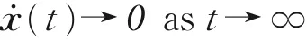
In addition，according to a classical result，L∞([0，∞ )，Rn)∩L2([0，∞ )，Rn)impliesast→∞.

（iii）From Eq.（11），we obtain

which gives immediately that

By differentiating the first equation of Eq.（11），we obtain

which impliesy→0ast→∞by noticing thatη＞0 andg(t)→0ast→ ∞.Thusx¨(t)→0ast→ ∞.

（iv）By using Eq.（11）again，we have

（v）Define

By elementary calculations，we derive that

which implies that（by noting

or

Integrate the above equation on[0，T]to obtain，together with the non-negativity ofE(t)

Due to properties（i）—（ii），x(t)，x˙(t)are uniformly bounded，and so ish(t).Hence，lettingT→∞in Eq.（16），we obtain

SinceE(t)is non-increasing，we deduce that

Using Eq.（17），the left side of Eq.（18）tends to 0 whenT→∞， which implies thatorJ(x(t))-J(x†)=o(t-1)ast→ ∞.The proof is completed.

Case IIη(t)=(1+2s)/tandt0=1

Now，we consider the following evolution system

Proposition 2Letxbe the solution of Eq.（19）.Then，fors≥1，the following properties hold

Proof（i）DifferentiatingE(t)of Eq.（10）

and using the system（19）to give

The remaining proof for property（i）is similar to that for property（i）of proposition 1.

（ii）Like the statements in the proof of proposition 1，we havethe limitexists.Now we showL2([1，∞ )，Rn).To the end，define

By using the convexity inequalityJ(x†)≥J(x)+(∇J(x)，x†-x)for allx∈Rnand Eq.（19），it is not difficult to show that

Hence，fors≥ 1，(t)≤ 0and thusE1(·)is non-increasing.Together with the fact thatE1(t)≥0for allt≥ 0，the limitexists.

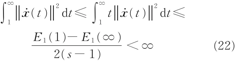
Integrating both sides in Eq.（21），we obtain that

（iii）From Eq.（19），we obtain

which gives immediately that

（iv）Define

By using the convexity inequalityand Eq.（19）again，we have

Similar toE1(·)，fors≥ 1，E2(·)is non-in-creasing，and the limiexists.Therefore，from Eq.（23），there holds

or

which givesJ(x(t))-J(x†)=O(t-2)ast→ ∞.The proof is completed.

Remark 1Compared with the first order method（6），where the convergence rate of the objective functional isJ(x(t))-J(x†)=O(t-1)，the convergence ratesJ(x(t))-J(x†)=o(t-1) in proposition 1 andJ(x(t))-J(x†)=O(t-2) in proposition 2 show that the second order dynamical systems（11）and（19）can achieve higher convergence order，indicating the second order dynamical system has a property of acceleration.

Now we are in a position to give the convergence result of the dynamical solutionx(t)of Eq.（7）with the noise-free data.Recall thatx†is the minimum norm minimizer of Eq.（4）with the exact datab.Then，formally，we have

where the superscript“+”means the Moore-Penrose inverse.

Theorem 2Letx(·)be the solution of Eq.（7）with the exact data，then

ProofLet{σj；uj，vj}∞j=1be the singular system for matrixA，i.e.we haveAvj=σjujandATuj=σjvjwith ordered singular values‖ ‖A=σ1≥σ2≥ …≥σr＞ 0.

Let’s first consider the case with fixed damping parameterη.Similar to Ref.［32］，we distinguish three different cases：（a） The overdamped case：η＞2‖ ‖A，（b）the underdamped case：there is an indexj0such that2σj0+1＜η＜ 2σj0，and（c）the critical damping case：an indexj0exists such thatη=2σj0.For simplicity，we only consider the overdamped case.The other two cases can be studied similarly.According to Ref.［32］，we have

where

Together with theorem 1，it is straightforward to check thatx(t)defined Eq.（25）is a unique solution of Eq.（11）.Moreover，we can deduce from Eq.（25）thatx(t)→(ATA)+ATbast→∞by noting that

Next we consider the case with dynamic damping parameterη(t)=(1+2s)/t.According to Ref.［35］，we have（note thatx˙0=0）

where

Γ(·)andJs(·)denote the Gamma function and the Bessel function of first kind of orders，respectively.As in the first case，x(t)defined in Eq.（27）is the unique solution of Eq.（19）.By using the asymptotic

for any fixedλ＞ 0， we conclude thatx(t)→(ATA)+ATbast→∞.The proof is completed.

1.3 Regularization properties for the noisy data

In section 1.2，we study the limiting behaviors of the solution for the second dynamical system（7）with noise-free data.It is shown that for exact datab，theoretically，the larger the timetis，the more accurate the solutionx(t)is.Therefore，we are readily given a satisfactory approximate solutionx(T*)tox†for a large enough timeT*.However，due to the inevitable noise，practically，it is not the case.In the case that only a noisy databδis available，the system（7）cannot produce a reasonable approximate solution unless the terminating timeT*is chosen appropriately.In other word，the asymptotic process should be terminated in advance.

In this subsection，we investigate the regularization property of the dynamic solutionxδ(t)of system（7），equipped with the Morozov’s discrepancy principle for selecting the terminating timeT*.

We define the Morozov’s discrepancy function as

wherexδ(t)is the solution of system（7），andτa fixed positive number.

Proposition 3For anyτ＞0，let the initial guessx0ischosen satisfyingThenχ(T)has at least one zero point.

ProofFirst，by theorem 1，it is easy to conclude thatχ(·)is continuous over[t0，∞ ).Recall thatxδis the minimum norm minimizer of Eq.（4）.Then，formally，likex†we have

Applying theorem 2 toxδ(t)yield

which implies

Now we are in a position to present a convergence result in the following.

Theorem 3Letxδ(t)be the solution of the dynamic system（7）.Denote byT*=T(δ，bδ)the first zero point ofχ(T).Thenxδ(T*)converges tox†inRnasδ→0.

ProofAsδ→0，T(δ，bδ)may go to infinity or may have a finite accumulation point.We first consider the situation thatT(δ，bδ)→∞.Recall thatAis am×nmatrix with the rankr.We proceed to the proof with two possible cases：（i）r≥n；（ii）r＜n.

（i）In the case ofr≥n，ATAis full rank，and thus

By using triangle inequality，

On one hand，by applying the convergence in theorem 2，we have

On the other hand，from Eq.（32）

Combine Eqs.（33）—（35）to conclude that

（ii）For the caser＜n，both the systems（1）and（3）have infinite solution，andx†，xδare the minimum norm solutions，respectively.Let{δn}be a sequence converging to 0 asn→ ∞，and letbδnbe a corresponding sequence ofnoisy data withFor a pair of(δn，bδn)，denote bythe corresponding terminating time point determined from the discrepancy principlesχ(T)=0.According to the continuity ofxδn(t)，for anyε＞ 0and large enoughnand thusT*n，there exists a pointT＜T*nsuch that

From the continuity ofxδn(·)due to theorem 2，for large enoughn，there holds

Moreover，by applying theorem 2 again，we obtain，for large enoughT（becauseT*ncould be large enough）

Then by combing Eqs.（36）—（38） and using triangle inequality

There is a numbern1such that for anyn≥n1

Sinceεis arbitrary，we arrive at the convergence of

For the case thatT(δ，bδ)has a finite accumulation point，we can use arguments similar to those in Theorem 2.4 of Ref.［36］，and omit here.The proof is completed.

2 Iterative Schemes

For the numerical implementation，this section is devoted to present several iterative schemes for the resolution of problem（4）.To the end，we first convert the system（7）into

or

Then，the numerical discretization of the differential system（39）or（40）together with the discrepancy principle produces second order iterative regularization methods.The damped symplectic integrators are extremely attractive since these schemes are closely related to the canonical transformations［37］，and the trajectories of the discretized second flow are usually more stable for its long-term performance.Applying the symplectic Euler method to the system（39），we obtain the iterative scheme at thekth step.

wherexk=xδ(tk)，qk=q(tk)，and Δtis the stepsize.By elementary calculations，scheme（41）can be expressed as the form of following three-term semi-iterative method.

whereak=(1-Δtη(tk))andωk=(Δt)2.

For the high order Symplectic methods，the Störmer-Verlet scheme can be considered as

Like Eq.（41），the iteration（43）can also be rewritten in the form of Eq.（42），but with parameters

InRef.［35］，amodifiedStörmer-Verlet scheme is proposed as

with parameters

As indicated by theorems 2 and 3，theoretically，for the noise-free data or noisy data with small noisy level，the iteration should go far enough for a good enough approximate solutionxk.In this case，it requires long time behavior for the iteration.Keep in mind that we are solving ill-posed problems.Therefore，when the data contains noise with not small noisy level，the iteration should stop in advance before the solution gets worse.Therefore，the accuracy itself in the discretization of system（39）or（40）plays more important role than the requirement of the long behavior.We can apply high order Runge-Kutta methods for this purpose.As an example，the classical fourth order Runge-Kutta method is adopted as

We note that other Runge-Kutta methods are possible.

After the discretization，the regularization parameter is reduced to the iterative stepk.For the schemes（41），（43），（44）and（47），the Morozov’s discrepancy principle reads：find the smallestksatisfying

3 Numerical Results

Two numerical examples are presented to demonstrate the effectiveness of the iterative regularization methods（41），（43），（44）and（47）for the resolution of the system（3）.For the sake of simplicity，the symplectic Euler method（41）is termed as SE1 or SE2，corresponding to a constant or timedependent damping parameter respectively.Similarly，the Störmer-Verlet method is termed as SV1 or SV2， the Modified Störmer-Verletmethod is termed as MSV1 or MSV2，and the Runge-Kutta method is termed as RK1 or RK2.In the following experiments，the maximal iterative numberNmaxis set as 5 000.

For the comparison of the proposed methods with the existing work，we introduce such classical iteration methods as Landweber method，conjugate gradient method（termed as CG），ν-method and the Nesterov’s method.For the problem （3），the Landweber method（5）reads

with0＜Δt＜2/‖A‖2.Theν-method has the form

withμ1=0，ω1=(4ν+2)/(4ν+1)，k=1，2，…

wherex-1，x0are the initial values， andgk=AT(Axk-bδ).In Eq.（50），ωnormplays the role of normalization，and can be set as

The Nesterov’s method is defined by

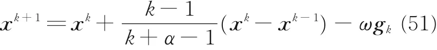
withα＞3，0＜ω≤ωnormandk=0，1，2，….

Like the methods in section 2，the Morozov’s discrepancy principle（48）is applied to Landweber method，CG method，ν-method and the Nesterov method for the choice of iterative numbers.

3.1 Example 1

In the first example，a Fredholm integral equation of the first kind of convolution type in one space dimension is considered as［38-39］

where the kernel functionk(x)=Cexp(-x2/2γ2)with positive constantsCandγ.Using numerical integration，Eq.（52）is discretized to a linear system as

Forhaving the data in the rightside of Eq.（53），we assume the exact solutionf†≡1.

Fig.1 Dependence of the condition number of the matrix K on n

Thend=Kf†，and the noisy data is constructed through

Then the noise level of the measurement data is calculated byδ=‖ ‖dδ-d.With matrixKand datad†，the iterative methods（41），（43）—（44），and（47）are applied to solve the noisy system

In all methods，we simply set the initial valuesf0=0，˙=0and the magnituden=100.For an approximate solutionfk，its accuracy is assessed by using the relative error as

In addition，IterN is used to denote iterative number where the iteration stops.

Fig.2 Dependence of IterN and L2err onΔt with η as a constant

The effect of the step-sizeΔton the iterative number and the solution accuracy is firstly investigated.To the end，fixδ′=1%，τ=1.03.The results are shown in Figs.2 and 3.Fig.2 corresponds to constant damping parameters（η=0.6for SE1，η=0.8for SV1，η=0.1for MSV1 andη=0.1for RK1）while Fig.3 corresponds to a variable damping parameter（η(t)=4/tfor all methods）.It is concluded that for all methods，on one hand，the largerΔtis，the faster the iteration is；on the other hand，its too big values may lead to the divergence.In the following experiments，we setΔt=0.7for SE1，Δt=0.8for SV1，Δt=0.4for MSV1，Δt=1.1for RK1，Δt=0.6for SE2，Δt=0.8for SV2，Δt=0.4for MSV2，Δt=1.1for RK2.They are all approximately optimal.

Fig.3 Dependence of IterN and L2err onΔt with η(t)=4/t

Next we investigate the effect of the parameterτ，used in discrepancy principle，on the iterative number and the solution accuracy.For this purpose， fixδ′=1%.The results are plotted in Figs.4 and 5 which show that on the whole，the larger the value ofτis，the less the iterative number is and the worse the solution accuracy is.In the remaining part，without specific statement，we setτ=1.03.

Fig.4 Dependence of IterN and L2err on τ with η as a constant

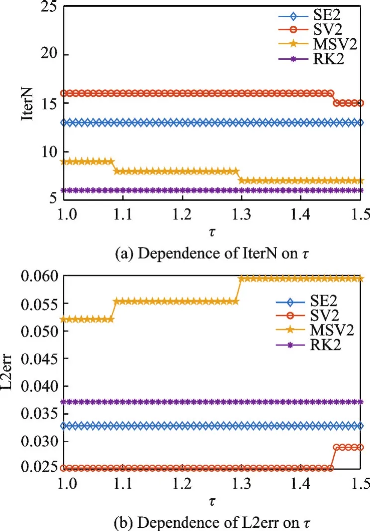
Fig.5 Dependence of IterN and L2err on τ with η(t)=4/t

We further compare the iterative schemes with the existing Landweber method，CG method，νmethod and Nesterov method.We setΔt=0.3for Landweber method，α=3，ω=0.16for Nesterov method，Δt=0.7，η=0.6for SE1，Δt=0.8，η=0.8for SV1，Δt=0.4，η=0.1for MSV1，Δt=1.1，η=0.1for RK1，Δt=0.6for SE2，Δt=0.8for SV2，Δt=0.4for MSV2，Δt=1.1for RK2.Moreover，setτ=1.03in all methods.The iterative numbers and relative errors in approximate solutions for different methods and different noise levels are given in Table 1，from which we conclude that with properly chosen parameters，all the mentioned methods are stable and can produce satisfactory solu-tions.Compared with the Landweber method，all the other mentioned methods have acceleration effect.On the whole，for all methods，the larger the noise level is，the worse the solution accuracy is，but the less the required iterative number is.Compared with SE1，SV1，MSV1 and RK1 methods，SE2，SV2，MSV2 and RK2 have better behavior，such as fewer iterative steps or better solution accuracy.Particularly，Table 1 shows that RK2 possesses the best behavior in both the iterative number and solution accuracy.

Table 1 Comparison between different methods in Example 1

Finally we study the effect of the magnitude of the problem on different iterative schemes.We fixδ′=1%，τ=1.03.The experimentsfor Landweber method，ν-method，Nesterov method and RK2 areimplemented repeatedly to solve Eq.（54）withn=25，50，100，200，400，800，1 600 and 3 200，respectively，and the results are shown in Fig.6.It is indicated from the Fig.6 that when the order of the matrix increases，the accuracy of the solution and the number of iteration steps change little.Moreover，Fig.6 also makes it clear that the RK2 performs better than three existing methods，especially when the scale of the problem increases.

Fig.6 Dependence of IterN and L2err on the scale n

3.2 Example 2

In the second example，the well-known illposed Hilbert matrix is taken to model the operator as

The dependence of the condition number of the matrixAon its scale is plotted in Fig.7，which shows that the condition number ofAincreases dramatically and thusAis ill-posed.Morevoer，like Example 1，assume again the exact solutionx†=(1，1，…，1)Tand computeAx†for the right sideb.The noisy databδis constructed like Example 1.Then iterations（41），（43）—（44）and（47）are applied to solve

Fig.7 Dependence of condition number of A on the scale n

Fig.8 Dependence of IterN and L2err onΔt with η as a constant

Fig.9 Dependence of IterN and L2err onΔt with η(t)=4/t

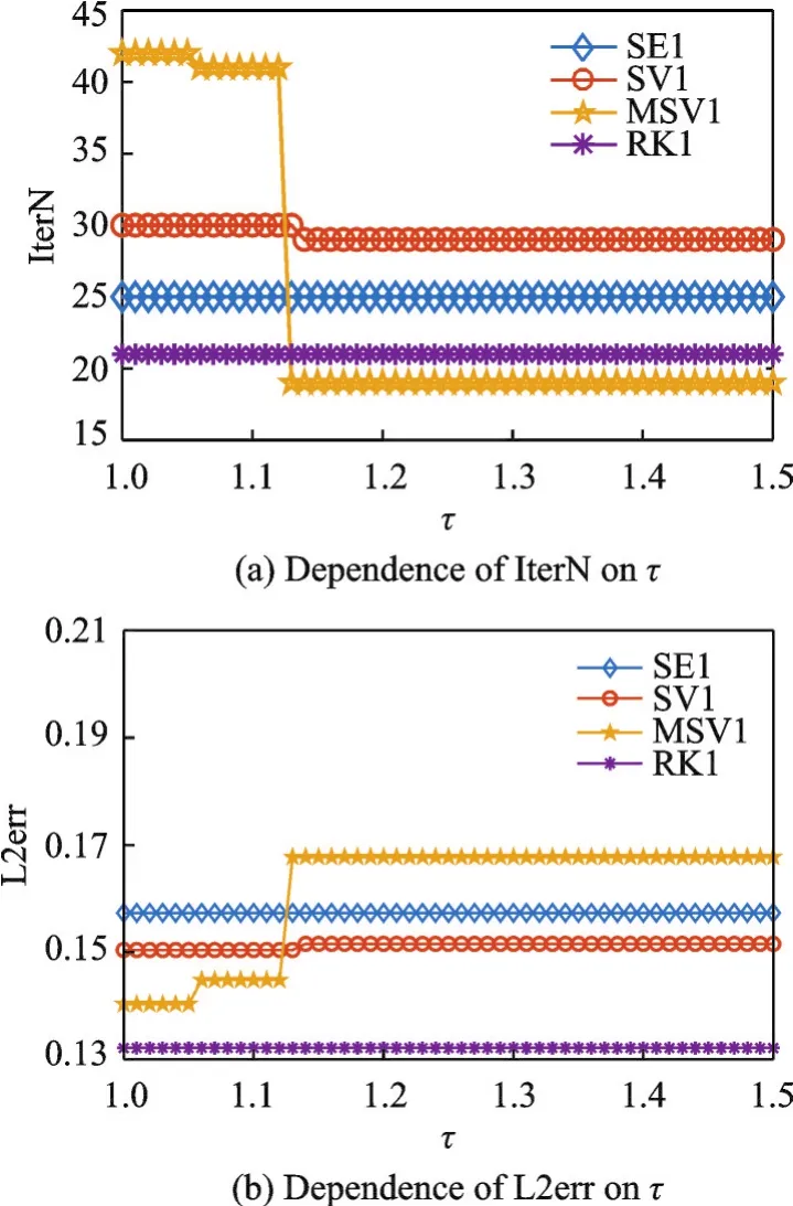
Fig.10 Dependence of IterN and L2err on τ with η as a constant

The dependence of the iterative numbers and the accuracy in approximate solutions obtained with iterations in Section 3 on parametersΔtandτare plotted in Figs.8—11.Specifically，Fig.8 is for constantη（withη=0.2for SE1，η=0.2for SV1，η=0.1for MSV1，η=0.1for RK1）while Fig.9 is forη(t)=4/t（both withτ=1.03）；Fig.10 is for constantη（with Δt=0.8，η=0.2 forSE1， Δt=0.9，η=0.2 forSV1， Δt=0.5，η=0.1forMSV1， Δt=1.2，η=0.1for RK1）while Fig.11 is forη(t)=4/t（ with Δt=0.7for SE2， Δt=0.9for SV2， Δt=0.5for MSV2，Δt=1.1for RK2）.In all figures，δ′=1%.Similar conclusion to those for Example 1 can be drawn from these figures.

Fig.11 Dependence of IterN and L2err on τ with η(t)=4/t

Similar to those in Example 1，a comparison between different methods for different noise data is displayed in Table 2，whereΔt=0.3for Landweber method，α=3，ω=0.2for Nesterov method，Δt=0.8，η=0.2for SE1， Δt=0.9，η=0.2for SV1，Δt=0.5，η=0.1for MSV1，Δt=1.2，η=0.1for RK1，Δt=0.7for SE2，Δt=0.9for SV2，Δt=0.5for MSV2，Δt=1.1for RK2.Also，τ=1.03in all methods.It can be concluded from Table 2 that with properly chosen parameters，all the mentioned methods are stable and can produce satisfactory solutions.

Table 2 Comparison between different methods in Example 2

The effect of the problem magnitude on different iterative schemes is also studied.The experiments for Landweber method，ν-method，Nesterov method and RK2 are implemented repeatedly to solve Eq.（55） withδ′=1%，τ=1.03，andn=25，50，100，200，400，800，1 600 and 3 200，respectively，whose results are shown in Fig.12.Again we can see from Fig.12 that the RK2 performs the best when compared with the existing classical methods.

Fig.12 Dependence of IterN and L2err on the scale n

4 Conclusions

The newly developed second order asymptotic system is applied to solve severely ill-posed linear system.Compared with the existing work，a series of theoretical results are presented and proved with simplified arguments.Since the existing work for second order system often assumes that it has exact solution while our problem may have no solution，the analysis is adjusted.On the whole，the fourth order Runge-Kutta method is better than the classicalν-method and Nesterov method，and much faster than Landweber method.Moreover，it is more obvious when the scale and the ill-posedness of the system increase.The reason is that the system is illposed and iteration should stop in advance before the accuracy gets worse.Therefore，although it is not a symplectic method，it has high precision.This is a new sight.Better behavior can be expected if higher precision scheme is used.The idea can also be applied to other linear inverse problems such as inverse source problems and Cauchy problems etc.，which will be studied in the future.