Predicting cutaneous leishmaniasis using SARIMA and Markov switching models in Isfahan, Iran: A time-series study
2021-01-22VahidRahmanianSaiedBokaieAliakbarHaghdoostMohsenBarouni
Vahid Rahmanian, Saied Bokaie✉, Aliakbar Haghdoost, Mohsen Barouni
1Department of Food Hygiene and Quality Control, Division of Epidemiology & Zoonoses, Faculty of Veterinary Medicine, University of Tehran,Tehran, Iran
2HIV/STI Surveillance Research Center, and WHO Collaborating Center for HIV Surveillance, Institute for Futures Studies in Health, Kerman University of Medical Sciences, Kerman, Iran
3Health Services Management Research Center, Institute for Futures Studies in Health, Kerman University of Medical Sciences, Kerman, Iran
ABSTRACT
KEYWORDS: Leishmaniasis; Climate factor; Time series analysis;Forecasting; Iran
1. Introduction
Leishmaniasis is a neglected vector born disease caused by the protozoan parasites of genus Leishmania that occurs in three forms, i.e. cutaneous, mucosal, and visceral forms[1]. Cutaneous leishmaniasis (CL) has been reported with an approximately annual incidence between 0.7-1.2 per million new cases worldwide.More than 90% of the CL cases have occurred in 8 countries, i.e.Afghanistan, Algeria, Brazil, Peru, Saudi Arabia, Syria, Iraq, and Iran[2].
According to the Ministry of Health and Medical Education of Iran,annually, about 30 000 cases of CL occurred in Iran. However, the number of actual cases is estimated to be four to five times[3]. There are two types of CL namely anthroponotic (ACL) and zoonotic CL(ZCL) in Iran. The ACL type is caused by Leishmania (L.) tropica,whose main reservoir is human and the vector is Phlebotomus (P.)sergenty[4]. The ZCL type is caused by L. major and the rodents including Rhombomys opimus, Meriones libycus, and Meriones nesokia are considered as the main reservoir. The main vector of the ZCL is P. papatasi[5,6]. This type is the most prevalent and has been found in 25 of 31 provinces in Iran, including Isfahan province as the oldest endemic foci of ZCL with the highest incidence in Iran[7].
Notwithstanding, the extensive public health activities have focused on prevention and control in surveillance systems; hence it was found that Isfahan had the highest mean incidence of CL between 1983 and 2013[3,4]. Several studies have reported the relation between CL and environmental factors such as rainfall, air temperature, slope of area, wind speed, evaporation rate, relative humidity, and vegetation cover[8-10]. A few studies have considered the effect of climate and environmental factors in time series analysis for modelling and prediction of CL in Iran.
Establishing a monitoring and surveillance system is necessary for both rapid detections of leishmaniasis outbreaks and for the monitoring of possible epidemics. Also, the public health system,especially in endemic areas, should be fully prepared to plan for potential outbreaks. Therefore, it is very important to use the models to predict the occurrence of leishmaniasis, especially in areas with high incidence. One of the most common models used in epidemiology is data analysis of time series. The purpose of using this method is to predict future values and the factors influencing its occurrence over time. Different models in time series analysis such as Gray models, general regression model, Box-Jenkins models,and negative binomial regression and neural network have been used to describe the pattern and predict the incidence of infectious diseases[11-13]. Each of these has its own considerations and accuracy.
In recent years, Box-Jenkins seasonal autoregressive integrated moving average (SARIMA) models have been used in medicine.Because infectious diseases fall into one of two stages of epidemic or non-epidemic and the use of these methods for early detection of outbreaks has limitations[14]. The use of mixed models in this case seems to be superior to models that use a single distribution for all observations[15]. Therefore, the objectives of this study are:(1) to determine the potential effect of environment variables on CL occurrence using time-series models, and (2) to compare the predictive ability of Markov switching model (MSM) and Box-Jenkins SARIMA models.
2. Materials and methods
2.1. Study site
Isfahan province is located in the center of Iran in the Zayandeh-Rud River of green plain, at the foothills of the Zagros mountain.The province had a population of 5 120 850 (4 507 309 urban and 613 073 rural area) according to General Population and Housing Census in 2016. The ancient and major city of Isfahan is the center of the province, making it the third-largest city in Iran. It also consists of 25 counties with an average altitude of 1 590 meters above sea level. The annual average of the minimum and maximum temperatures in this province is 10 ℃ and 25 ℃, respectively. The climate in this area is highly variable so that the average annual rainfall is between 100 and 150 mm. The air humidity is in the range of 11% to 82% and the average number of hours of sunshine per month is 260 hours.
2.2. Data collection
This descriptive study employed yearly and monthly data of 49 364 parasitologically-confirmed cases of CL in Isfahan province between January 2000 and December 2019. The data were provided by the leishmaniasis national surveillance system at Isfahan University of Medical Sciences.
All climate and weather data such as the average monthly temperature (℃), average monthly maximum and minimum temperature (℃), average monthly pressure (p), average monthly relative humidity (%), average maximum and minimum relative humidity (%), total hours of sunshine per month, total number of rainy days per month, total monthly rainfall (mm), number of days with dust, maximum and minimum monthly wind speed (km/h) were gathered from the meteorological organization of Isfahan province.The data were collected from 10 synoptic centres in Isfahan province, which shows the highest incidence of CL.
Vegetation information was extracted from the Moderate Resolution Imaging Spectroradiometer (16-day composites) satellite,which is accessible to the public. Moderate Resolution Imaging Spectroradiometer uses remote sensing data of the Normalized Difference Vegetation Index (NDVI) for analysis, measurement,and evaluating the presence or absence of vegetation in an area. The range of NDVI changes is between +1 and -1, where negative values of the index (numbers close to -1) indicate water zones. The values close to zero (between -0.1 and +0.1) usually indicate bare rock,sand, or snow surfaces. Low and positive values of the index (about+0.2 to +0.4) indicate vegetation of shrubs and grasslands, and high values of NDVI (numbers close to +1) indicate dense vegetation(dense green forests)[16]. The NDVI data of the province were accessible via the website of the Iranian Space Agency for the period between January 2000 and December 2019[17]. Before choosing any model, the trend of CL incidence and environmental variables were observed by plotting data and these plots showed the seasonal trend with periodicity. Also, due to the sinusoidal wave of the coefficients and the significance of the correlation in the lags of 12, 24, and 36 months, it seems that the occurrence of CL and environmental variable does have a seasonal pattern. Therefore, the SARIMA model was selected.
2.3. Statistical analysis
2.3.1. SARIMA model
The monthly occurrences case during the period of this study constructed the SARIMA model. This model is described by seven parameters including SARIMA (p,d,q), (P,D,Q), and s where p is the number of autoregressive, d is the number of times the model was differenced, q is the number of moving averages, P is the number of seasonal autoregressive, D is the number of seasonal integration or seasonal differencing, Q is the number of seasonal moving average,and s is the length of seasonal periods[8].
To check the stationary in variance and mean, Box-Cox regression and Dickey-Fuller test were applied, respectively. To eliminate seasonality trend, the first-order seasonal differencing (D=1) with a period of 12 was used. For estimation of the moving average and autoregressive parameters, autocorrelation functions (ACF) and partial autocorrelation functions (PACF) were identified[18].
In the next step, Akaike information criteria (AIC) lower, Bayesian information criterion (BIC), and likelihood ratio test among possible models showed a better approach among models which were expanded by different lags[15,19]. Finally, a SARIMA (1,0,1)(1,1,1) 12 model was selected with the lower AIC (197.35) and BIC (225.17) values to fit the data in the best way.
Independent variables as external regress with different lags were observed in relation to CL cases using cross-correlation coefficients to detect the best predictor; hence its best lags were included in the final multi-regression SARIMA model.
Later, the achieved SARIMA model was applied to predict the frequency of monthly occurrences case. The forecasting precision was estimated by the mean absolute percentage error (MAPE),which was computed using equation (1). The lower the value, the higher the accuracy of the fitted model.

Where N is the number of predictions.
Furthermore, to measure the goodness-of-fit of the final model, the portmanteau test was run for white noise and the normality of the residuals was observed on the graphs[19].
2.3.2. MSM
The simple time series models cannot explain nonlinear occurrence of outcomes such as the data of surveillance system of infectious diseases, therefore the MSM model is used due to the problem of structural failure and nonlinearity of series[15]. MSM model is one of the most popular for nonlinear time series models that shows the occurrence of outcomes in different states[14].
Since the CL series has a switching state from epidemic and nonepidemic and vice versa (as the name of the switching suggests),therefore this model was found suitable for analysing and predicting such data. In this study, modeling is done separately for the epidemic and non-epidemic state.
A simple MSM model can be written as follows (in this model, S=1 means epidemic state and S=0 means non-epidemic state):

This model shows that in the non-epidemic state S=0 and the value of yis determined based on aconstant and the autoregressive parameter with a. If an epidemic occurs (S=1), the constant value increases to a+ aand the autoregressive parameter value increases to a+ a(Equation 2).
Equation 3 shows that the hidden states Sis a function of Markov significant with the transition probability. Pis the probability of state j at time t conditional to state i at time t-1:

The transition matrix is also an N*N matrix consisting of P. After fitting the model and estimating the parameters, the values of pand pwere also estimated. According to the values of these parameters,the matrix of transition probabilities can be formed as follows:

In this matrix, the sum of the probabilities of each row is equal to one. Here, pmeans that the regime is likely to be at non-epidemic state at time t, provided it is at non-epidemic state at time t-1. The pmeans the probability that the regime will be in a state of epidemic at time t, provided that it is also in a state of epidemic at time t-1. The pmeans the probability that the regime is in a state of epidemic at time t, provided that it is at non-epidemic at time t-1. The means pthe probability that the regime is in a non-epidemic state at time t,provided that it is in a state of epidemic at time t-1. To control the seasonality trend, the parametric method of periodic function (Fourier terms) was used. In this method, Sinus and Cosinus functions of time(according to the period of the seasonal pattern based on the data)were entered into the model along with other variables. Also, other independent variables may enter the model with lag or different delays (here environmental variables), in which case the final model is written as follows:


The validity of the MSM was also examined by fitting the data for the period of the study. Nonetheless, the final SARIMA and MSM models were compared based on AIC, BIC, and MAPE indices. Data analysis was performed using Stata software (version 14) and the package time series analysis. The alpha level was 0.05.
2.4. Ethical considerations
The study was conducted in accordance with the Declaration of Helsinki, and the protocol was approved by the Faculty of Veterinary Medicine, University of Tehran, Iran (Project identification code:7265130).
3. Results
3.1. Descriptive analysis
A total of 49 364 cases of CL have been reported in Isfahan province between 2000 and 2019. Figure 1 shows that the trend of CL is seasonal. There is a clear increase in the number of cases from 2011 to 2015, then this starts to decline in 2015 while again it follows an upward trend in 2018. The CL trend is almost stable from January to June. Then it starts to climb from July and reaches its peak in September and October and then starts to decline (Figure 2).Figure 3 shows the trend of significant environmental data between January 2000 and December 2019 in Isfahan province that was used for modelling.

Figure 1. The trend and distribution of 49 364 cutaneous leishmaniasis cases between January 2000 and December 2019 in Isfahan province.

Figure 2. Monthly cumulative distribution of the number of cutaneous leishmaniasis cases in Isfahan province between 2000 and 2019.
3.2. Cross-correlation function
Table 1 shows that there are cross-correlation coefficients and a significant level of CL incident with the average relative humidity at lag of 2 months, maximum relative humidity at lag of 2 and 8 months, minimum relative humidity at lag of 2 months, minimum wind speed at lag of 0 and 8 months, maximum wind speed at lag of 0, 1, 2, and 3 months, total hours of sunshine at lag of 2and 3 months, number of days with dust at lag of 7 months, mean NDVI at lag of 0, 9 and 11 months. However, there is no significant correlation between other variables and the incidence of CL in any of the lags. Zero lags were not considered due to its insignificance and non-applicability.

Table 1. Cross-correlation coefficients of environmental variables in Isfahan province from zero lag (communication without delay) to 12 months’ lag.

Figure 3. The time series and trend of environmental data between January 2000 and December 2019 in Isfahan province.
In the next step, due to the possibility of collinearity between independent variables in significant lags, Pearson correlation coefficient was used and if there is a strong correlation (above 0.7)between independent variables, one of them was entered the model. There is a strong correlation between the average relative humidity at lag of 2 months with the maximum relative humidity at lag of 2 months (r=0.84), the minimum relative humidity at lag of 2 months (r=0.88), total hours of sunshine at lag of 2 months(r=-0.72) and total hours of sunshine at lag of 3 months (r=-0.92).Therefore, it was decided not to enter the average relative humidity at lag of 2 months in the model. On the other hand, there was a high correlation between the maximum relative humidity at lag of 2 months with total hours of sunshine at lag of 2 months (r=-0.87)and the minimum relative humidity at lag of 2 months with total hours of sunshine at lag of 3 months (r=-0.76). It was decided not to include total hours of sunshine at lag of 2 and 3 months in the model(Table 2). Finally, with the above considerations, the following was entered to the model: maximum relative humidity at lag of 2 and 8 months, minimum relative humidity at lag of 2 months, minimum wind speed at lag of 8 months, maximum wind speed at lag of 1, 2,and 3 months, number of days with dust at lag of 7 months, and the mean NDVI at lag of 9 and 11 months.

Table 2. Pearson correlation coefficient between independent variables in significant lags.
3.3. SARIMA model
Initially, the above independent variables were entered into the model as univariate, and finally, independent variables with a P-value of less than 0.2 were entered into the model as multivariate. Also,the non-significant variables of multiple models were removed one by one from the model (backward method) and the models were examined with Likelihood ratio test.
Finally, the best-fit model with the lowest AIC and BIC values,the standard error, and 95% confidence interval of coefficients and significance was selected (Table 3).
According to Table 3, CL is significantly associated with the variables of minimum relative humidity at a lag of 2 months, and maximum wind speed at lag of 3 months. The minimum humidity variable with a significantly low value (P=0.002) seems to be the most important variable involved in the fluctuations of CL. The vegetation cover at a lag of 9 months, is present in the model and has the highest coefficient value (-4.64). The presence of this variable in the model improved the AIC but has not shown a significant association with CL incidence (P=0.07).
The AIC and BIC values of model with explanatory variables were less than the model without explanatory variables. Also, the calculated value of MAPE was 11.45%.
To confirm the goodness of fit of the model, the residuals(differences between actual cases and predicted cases) were compared. The histogram of the residues showed that the residues follow the normal distribution. Moreover, the portmanteau test confirmed the residuals normality and independence (P=0.89).
Figure 4 shows the fitted cumulative number of CL cases between January 2000 and December 2019. To evaluate the validity of the model, we showed the fitted model with actual data of CL between January 2000 and December 2019, and then predicted the number of CL cases with 95% confidence intervals between January 2020 and December 2021, based on the final best- fit model. The predicted model was completely fitted to the actual data (Figure 4).
3.4. MSM
In MSM model, similar to the SARIMA model, at the beginning of preparing the series or data to fit the model, Box-Cox regression test was used to check the stationary in variance of the data. This test showed that CL data were not stationary in variance and therefore according to the value of theta (theta=0.08), a log transformation was used. Autocorrelation and partial autocorrelation plots and Dickey-Fuller test (P≤0.001) showed that the data are stationary in the mean.
In this study, because modelling is for an infectious disease, two regimes (state=2) were considered for modelling. State 0 was considered for the non-epidemic regime and state 1 was for the epidemic regime. Table 4 lists the results of the fitting to MSM model.

Table 3. Parameter coefficients of simple and multiple SARIMA (1,0,1) (1,1,1) 12 model for cutaneous leishmaniasis cases in Isfahan province (seasonal differencing was used for seasonality control).

Figure 4. Observed cutaneous leishmaniasis cases between January 2000 and December 2019 and 1-step ahead predicted values between January 2020 and December 2021 based values on the multiple SARIMA (1,0,1) (1,1,1) 12 model with 95% confidence intervals.
If we consider the constant estimated by the model in epidemic state as the epidemic threshold, and according to this model, the number of cases above 108 cases for CL in the province per month can be considered as the outbreak threshold. This is because log transformation was used to stationary the variance of the series, and the exponential of this coefficient was used to reach the real value,so that exp (4.68)=108.12.
Also, as the constant variance is higher in non-epidemic state, so it can be concluded that the number of cases in the non-epidemic period has more fluctuations than the epidemic periods.
In addition, according to the simple MSM, the transition probabilities were calculated as follows:

Pis indication of the non-epidemic state. It is 93.5% likely to stay in non-epidemic state, and only 6.5% is likely to change from a nonepidemic to epidemic state. Pindicates a 1.7% chance of regime change from epidemic to non-epidemic state. In other words, if the regime is in an epidemic state, it is 98.2% likely to stay in epidemic state.
The following equations were used to calculate the average period in each regime:
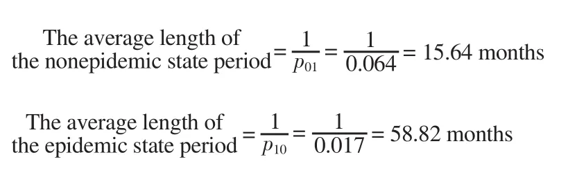
That is, when the regime is in the non-epidemic state, it lasts an average of 15 months, and when it enters the epidemic state, it lasts an average of 58 months, and then enters a non-epidemic state.
The multiple MSM shows that among the environmental variablesincluded in the model, the variable of minimum wind speed at a lag of 8 months (P<0.001) has an effect on the non-epidemic state.

Table 4. Regression coefficients of simple and multiple MSM for cutaneous leishmaniasis cases in Isfahan province [Seasonality controlled with the parametric method of periodic function (Fourier terms)].
The variables of relative humidity maximum at a lag of 8 months(P=0.032), the minimum wind speed at a lag of 8 months (P<0.001),the maximum wind speed at a lag of 1 month (P=0.005), and the maximum wind speed at a lag of 2 months (P=0.029) were significantly associated with CL epidemics. The MSM estimated with the environmental variables was a better fit than the simple MSM model (without independent variables), with the lowest AIC value (Table 4).
Figure 5 shows the number of observed and predicted CL cases for the period between January 2000 and December 2019 based on the multiple MSM. The predicted model was completely fitted to the actual data (Figure 5). Also, the calculated MAPE was 3.5%.

Figure 5. The observed and predicted cutaneous leishmaniasis cases between January 2000 and December 2019 based values on the multiple MSM.
3.5. Comparison of SARIMA and MSM models
Comparing both simple and multiple SARIMA models with simple and multiple MSM, it can be seen that AIC, BIC, and MAPE in MSM are much smaller than SARIMA models. Regarding the correlation between environmental variables in the SARIMA model,it was observed that there was significant association of CL cases with the variables of minimum relative humidity at a lag of 2 months and maximum wind speed at a lag of 3 months. While in the MSM,there was significant association of CL cases with the variables of maximum relative humidity at a lag of 8 months, minimum wind speed at a lag of 8 months, maximum wind speed at a lag of 1 month, and maximum wind speed at a lag of 2 months. However,the advantage of MSM is separating the effect of the independent variables individually in the epidemic and non-epidemic state, which in turn can provide the policymaker with the transition probabilities and the duration of each state.
4. Discussion
Time series analysis of surveillance data on infectious diseases is important to stimulate new hypotheses, predict observed events, and subsequently establish a quality control system[18,20]. The results of this study showed that the trend of CL is seasonal. The trend started to increase in July and reaches its peak in September and October and then starts to decline. This result can be justified considering the biology of vector (sand flies) and activity of reservoir (rodents)of Isfahan province[3,10]. Thus, in this province, the activity of P. ansari, P. sergenti, P. caucasicus, and P. papatasi as the main vectors of CL in Isfahan, continues from early April to August and the activity of Rhombomys opimus as the main reservoir is in spring and summer[3,21]. According to the extrinsic incubation period in sand flies (3 days) and incubation period in humans (approximately 4 months), it is compatible with the CL trend in this region[8,22].
Furthermore, our finding showed that the CL is in an epidemic state for 58 months, and a 15-months period of non-epidemic state with a recurrence of five years enters the epidemic stage. Therefore, it can be concluded that the interventions that have been made to control the disease for 20 years have not been very effective and the disease has gone through its normal course.
In the recent study which focused on Isfahan province between 2007 to 2015, there is no indication of CL incidence, and the incidence had been decreased by the end of the study[10]. This discrepancy in results can be attributed to the fact that this study considered the unit of time as year in eight time periods, while in the present study the period as month in 240 time periods (20 years)studied.
The results of this study are based on two reliable time series models that showed that minimum relative humidity, maximum relative humidity, minimum wind speed, and maximum wind speed were significantly associated with CL epidemics in different lags(P<0.05).
Numerous researches conducted in Iran have shown an association between environmental factors and CL occurrence. In a study conducted in Isfahan province by Ramezankhani et al. using negative binomial regression method, they showed that there is a significant association of mean temperature, relative humidity, land slope,maximum wind speed, rainfall, altitude, and vegetation with the incidence of CL[23]. Also, a similar study using the SARIMA time series model run in Fars province of Iran showed that the rainfall,relative humidity, and rainy days are associated with the incidence of CL[8]. Similar results were reported in Golestan Province, Iran[24].There are reported studies in other parts of the world such as Tunisia[25], Tanzania[26], Algeria[27], and Afghanistan[28]. All of these found that there is a positive correlation between rainfall, humidity,and mean temperature with the incidence of CL. These effects can be explained due to the impact of these factors on the spread, survival,and activity of Leishmania parasite, its reservoirs, and vectors of this disease. Increasing the population of sandflies can increase the number of bites and consequently increase the transmission of infection. Increasing the minimum temperature and humidity reduces the maturation period and the extrinsic incubation period in sand flies, which can increase their population and consequently the rate of infection transmission[29,30]. In addition, female sand flies usually choose places with high humidity and temperature to lay their eggs so that their larvae can have the required humidity and temperature for their survival to provide easy feeding conditions[8,31].The correlation between wind speed and some vector-borne diseases has been proven. Accordingly, wind has dual effects on the vectors and the hosts. A high-speed wind can reduce the possibility of mosquito bites; on the other hand, it can increase the flight length of sand flies[10,32].
In this study, we firstly performed pre-whitening to evaluate the relationships between the incidence of CL and the environmental data at different lags. Then, the cross-correlation between the residuals of SARIMA models in different series was investigated[8,15]. In time series analysis, cross-correlation on the original data is not recommended because without pre-whitening,the significant correlations observed between the one lags of different variables may be due only to the auto-correlation in seasonal time series[33]. In addition, the statistics such as Pearson and Spearman correlation coefficients assume that the data are independent, whereas this assumption is not true in time series data.Each observation is correlated with its previous values, so using such statistics without pre-whitening can result in a misleading outcome.
The relationship between environmental parameters and CL occurrence in different lags is attributed to the indirect occurrence of disease with sand fly activity at different times[29]. It is found that the CL is more common in autumn and winter, hence it is better to get more insight into this and how they are related. For example, with the noticeable change of environmental factors from a few months ago to the health system, there should be an alert about the epidemic of the disease, which in this study showed the models up to 8 months ago, i.e. at lag of 8 months.
In recent years, the use of ARIMA models in medicine and health,especially zoonotic diseases, has been increasing. Rahmanian et al.used the ARIMA (3,0,4) model to forecast human brocellosis in Yazd province, Iran[18]; Tohidinik et al. applied SARIMA (2,0,0) (2,1,0,12)models to forecast zoonotic CL in Fars province, Iran[8]. Yang et al.used ARIMA (0,2,1) to predict incidence of Malta fever in China[11]and Esmaeilzadeh et al. used ARIMA (1,0,0), ARIMA (1,0,1), and ARIMA (1,0,1) for determining the new confirmed cases, the death cases, and the recovery cases of COVID-19 in Iran[20].
The main idea of using Markov models in epidemiological surveillance of infectious diseases was established in 1999[34],but few studies have used the MSM to forecast zoonotic diseases,especially leishmaniasis. The results of this study showed that despite the relatively acceptable predictive power of SARIMA and MSM models, the latter provides more information to policymakers and is more helpful in planning for future interventions than the former model.
One of the strengths of this study is that the time unit considered is much longer than other time-series studies, i.e. 240 months, which reveals more accurate and detailed information about the trend of disease and its link with the environmental factors. Also, to our best knowledge, this is the first study that simultaneously uses the SARIMA and MSM of time series analysis for CL and compares them.
The limitations of this study lie in the fact that there are other parameters than the climatic factors such as host-related factors,vectors, reservoir diversity, parasite type, soil type, and health interventions performed in the epidemiology of CL in this region which are effective and should be considered for the future studies.In conclusion, the results of this study showed that SARIMA(1,0,1) (1,1,1) 12 model and MSM can be a useful tool for predicting CL in Isfahan province. The time-series models can be used as a complementary tool of national disease surveillance systems for early warning of epidemics. This can help policymakers as a decision support tool in the preparedness of public health problems before the start of epidemic of the disease.
Since infectious diseases fall into one of two states of epidemic and non-epidemic, the use of MSM (dynamic) in this case is recommended as it provides more information to model as compared to single distribution (Box-Jenkins SARIMA) for all observations.The MSM seems to be suitable for the disease which does not have a seasonal trend and their regime is changed in the long term.Therefore, we recommend that in future studies, this model should be applied for diseases that do not have a seasonal trend.
Conflict of interest statement
The authors declare that there is no conflict of interest.
Acknowledgements
This study was derived from Ph.D. thesis from faculty of Veterinary Medicine, University of Tehran, Tehran, Iran. The authors would like to thank health deputy of Isfahan University of Medical Sciences for trying to control these infections and perform primary health care.
Authors’ contributions
The initial idea of this study was by VR. SB and VR contributed to the design of the work, data collection and writing of drafting the article and implementing all comments from the reviewers. VR and AAH participated in the data analysis and interpretation. AAH and MB contributed to a critical revision of the article. All authors read and approved the version to be published.
杂志排行

Asian Pacific Journal of Tropical Medicine的其它文章
- Insecticide resistance status and biochemical mechanisms involved in Aedes mosquitoes: A scoping review
- Genomic characterization of velogenic avian orthoavulavirus 1 isolates from poultry workers: Implications to emergence and its zoonotic potential towards public health
- Molecular detection and genetic diversity of Dientamoeba fragilis and Enterocytozoon bieneusi in fecal samples submitted for routine parasitological examination
- Antimicrobial resistance patterns and prevalence of integrons in Shigella species isolated from children with diarrhea in southwest Iran
- Biofilm-forming fluconazole-resistant Candida auris causing vulvovaginal candidiasis in an immunocompetent patient: A case report