Evaluation of Arctic Sea-ice Cover and Thickness Simulated by MITgcm

Fei ZHENG, Yue SUN, Qinghua YANG, and Longjiang MU

1International Center for Climate and Environment Science, Institute of Atmospheric Physics,Chinese Academy of Sciences, Beijing 100029, China

2Collaborative Innovation Center on Forecast and Evaluation of Meteorological Disasters,Nanjing University of Information Science and Technology, Nanjing 210044, China

3University of Chinese Academy of Sciences, Beijing 100049, China

4School of Atmospheric Sciences, Sun Yat-sen University, and Southern Marine Science and Engineering Guangdong Laboratory (Zhuhai), Zhuhai 519082, China

5Alfred Wegener Institute, Helmholtz Centre for Polar and Marine Research, Bremerhaven 27515, Germany

ABSTRACT A regional Arctic Ocean configuration of the Massachusetts Institute of Technology General Circulation Model(MITgcm) is applied to simulate the Arctic sea ice from 1991 to 2012. The simulations are evaluated by comparing them with observations from different sources. The results show that MITgcm can reproduce the interannual and seasonal variability of the sea-ice extent, but underestimates the trend in sea-ice extent, especially in September. The ice concentration and thickness distributions are comparable to those from the observations, with most deviations within the observational uncertainties and less than 0.5 m, respectively. The simulated sea-ice extents are better correlated with observations in September, with a correlation coefficient of 0.95, than in March, with a correlation coefficient of 0.83.However, the distributions of sea-ice concentration are better simulated in March, with higher pattern correlation coefficients (0.98) than in September. When the model underestimates the atmospheric influence on the sea-ice evolution in March, deviations in the sea-ice concentration arise at the ice edges and are higher than those in September. In contrast,when the model underestimates the oceanic boundaries’ influence on the September sea-ice evolution, disagreements in the distribution of the sea-ice concentration and its trend are found over most marginal seas in the Arctic Ocean. The uncertainties of the model, whereby it fails to incorporate the atmospheric information in March and oceanic information in September, contribute to varying model errors with the seasons.

Key words: Arctic sea ice, MITgcm, simulation and evaluation, sources of model error

1. Introduction

Sea ice plays an important role in the Earth’s energy budget and has a substantial impact on local and remote atmospheric and oceanic circulations (e.g., Steele et al., 2008).Due to its high albedo, sea ice can maintain cooler polar temperatures by reflecting much of the incident sunlight back into space (e.g., Maykut, 1982). If warming temperatures gradually melt sea ice over time, fewer bright surfaces are available to reflect sunlight back into space, and more solar energy will be absorbed at the surface, which causes the air temperature to further increase and sea ice to be lost. This positive feedback process between sea ice and temperature makes the Arctic one of the most sensitive regions to global warming, contributing to Arctic amplification (Serreze et al., 2008). Since the increase in air temperature over the Arctic Ocean has exceeded the average temperature increase in the Northern Hemisphere, sea ice has undergone unprecedented decline in recent years (Overland et al., 2016). Many studies have shown that the reduction in the Arctic sea-ice cover could potentially influence the weather patterns and even the climate in the Northern Hemisphere (e.g., Francis and Vavrus, 2012; Liu et al., 2012, 2013; Cohen et al., 2014).For example, Hopsch et al. (2012) found that there is a mechanism of negative feedback between the North Atlantic Oscillation and sea ice. On the other hand, the formation and ablation of sea ice can directly change the salinity of seawater,which affects the surface buoyancy flux in deep-water-formation regions and further modulates the Atlantic thermohaline circulation (e.g., Holland et al., 2001). Miles et al.(2014) found that there exists an intrinsic link between seaice coverage and Atlantic multidecadal variability. Due to atmospheric and oceanic circulations, changes in the Arctic Ocean could further exert a widespread and far-reaching influence on human societies as well as animal habitats (e.g.,Regehr et al., 2010; Eicken, 2013). In addition, economic factors, such as increased tourism, resource exploration and the potential opening of sea routes in the Arctic Ocean, have drawn increasing attention; these activities would definitely benefit from reliable sea-ice simulations and predictions(Smith and Stephenson, 2013).

In light of the importance of sea ice for both scientific research and human activities, it is imperative to obtain a more comprehensive understanding with a reasonable prediction of the variability in Arctic sea ice at different time scales (Guemas et al., 2016). Fortunately, since satelliteobserved sea-ice data became available in the mid-1970s, it has been possible to continuously monitor the conditions of Arctic sea ice. However, to a certain extent, satellite observations do not allow scientists to optimally view sea ice in all conditions due to the limitations of the time span and spatial resolution or to explore the physical processes involved in the evolution of sea ice (Comiso et al., 2017). In this case, climate sea-ice models are feasible tools for simulating the evolution of Arctic sea ice and for investigating its impact on the climate (Stroeve and Notz, 2015). However,no model simulations can perfectly capture the behavior of the real world because the processes involved in sea-ice evolution are too complex to be described exactly by mathematical equations. According to the assessment of CMIP5,there remains considerable scatter in the modeled sea-ice extent, and the trends in sea-ice cover from most ensemble members and models are mostly lower than the observed values (Stroeve et al., 2012b). CMIP6 models still tend to simulate a wide spread of the mean sea-ice area and volume, and most models fail to simultaneously simulate a reasonable evolution of sea-ice area (SIMIP Community, 2020). These disagreements between the model simulations and observations could be the result of a combination of many underlying factors, including internal variability, the shortcomings of the sea ice-ocean model formulations, and the atmospheric and oceanic forcing of the simulated sea ice (Notz et al., 2016). Therefore, the reasonable simulations of sea ice by models should be compared to observations, and the sources of the model errors must be understood; this type of analysis is beneficial to the development of sea-ice models and leads to greater understanding of the significance of sea ice regarding the global climate.

In this study, we focus on the representation of the seaice concentration, sea-ice extent and sea-ice thickness to evaluate the performance of the sea-ice components simulated by the Massachusetts Institute of Technology General Circulation Model (MITgcm). Many studies based on a regional Arctic configuration of MITgcm have been performed to assess and improve sea-ice simulations. For example, Losch et al.(2010) presented sea-ice simulations from different model configurations and found that the dynamic solver has a greater effect on model performance than the boundary conditions, ice rheology, and ice-ocean stress coupling; Nguyen et al. (2011) attached importance to the uncertainties from model parameters and applied a green function approach to adjust a set of parameters for optimized simulation; Yang et al. (2014, 2016) improved the simulations of sea-ice concentration and thickness by data assimilation and presented important effects from the atmosphere on sea-ice simulation. These studies have demonstrated the good performance of MITgcm and investigated the possible sources leading to the uncertainties in the model results. However, most of these studies focused on evaluating the decadal variability or the trends of sea ice in simulations with MITgcm, and further estimations of the model’s performance regarding seasonal sea-ice simulations and the possible factors for model-observation disagreements in different seasons are needed.

In this work, we concentrate on evaluating aspects of Arctic sea-ice simulations in March and September: (1) the distribution of ice concentrations and the corresponding extents over the simulation period are assessed to determine how well the model captures the observed state of the sea-ice cover, and (2) the trends in the March and September ice extent and concentration are assessed to measure whether the model has the ability to capture the response of the Arctic sea ice to global climate change in different seasons (Stroeve et al., 2012b). Additionally, both the temporal and spatial distributions of the sea-ice thickness are discussed to assess the performance of the model. We then carry out further analysis on the relationship between the sea-ice extent and the boundary conditions, including the atmosphere and the ocean, to explore the possible sources of disagreements between the simulations and observations in March and September.

The structure of this paper is as follows: In section 2,we introduce the data and methods used for model simulation and evaluation. In section 3, the spatiotemporal variability of sea-ice cover and thickness are evaluated. In section 4, an analysis of the possible model error sources is performed. And finally, section 5 provides a discussion and conclusions.

2. Data and methods

2.1. Data

The Arctic configuration of MITgcm is similar to that used by Yang et al. (2014), more information on which can be found in the supplementary material. The simulation starts from climatological initial fields including temperature and salinity derived from the World Ocean Atlas 2005(Antonov et al., 2006; Locarnini et al., 2006). The lateral boundary conditions, including the monthly potential temperature, salinity and ocean currents, are derived from the Estimating the Circulation and Climate of the Ocean project,Phase II (ECCO2) (Menemenlis et al., 2008). The model is forced with six hourly atmospheric forcing variables, including 2-m air temperature, 2-m specific humidity, 10-m wind speed, downward shortwave radiation, downward longwave radiation, and precipitation, obtained from the Japanese 25-year Reanalysis Project (JRA-25) reanalysis data and the Japan Meteorological Agency Climate Data Assimilation System (Onogi et al., 2007). In addition, to further investigate the relationship between sea ice and atmospheric forcing, ERA-Interim, a global atmospheric reanalysis from 1979, is analyzed in section 4 (Dee et al., 2011).

The observations of sea ice chosen for the model-observation intercomparison studies are summarized in Table 1.As discussed in Notz (2014), the estimation of sea-ice concentration differs in different algorithms that derive the sea-ice concentration from the satellite data by different transfer functions. In this work, the simulations are compared with satellite retrievals of sea-ice concentration based on three algorithms—namely, the Bootstrap algorithm (Comiso,2017), the NASA Team algorithm (Fetterer et al., 2017) and the ARTIST Sea Ice (ASI) algorithm (Kaleschke et al.,2001)—to evaluate the performance of the model. Both the Bootstrap algorithm and NASA Team algorithm provide sea-ice concentration data from 1979 onwards and come from SMMR, SSM/I and SSMIS. The satellite retrievals based on the ASI algorithm provide the sea-ice concentration based on SSM/I from 1991 onward and based on AMSR-E data from 2002 onward. Based on the gridded data of sea-ice concentration, the sea-ice extent is calculated by adding the area of all grid cells with an ice concentration of more than 15%. Sea-ice thickness observations from different data sources, including ICESat, CryoSat2 and Operation IceBridge, are chosen for model evaluation.

2.2. Analysis method

It is well known that the root-mean-square deviation(RMSD) is a measure of the average distance between simulations and observations. The fact that the RMSD can be decomposed into several components makes it possible to determine the specific source of the difference between simulation and observation (Taylor, 2001). The decomposition of RMSD is defined as

where R ≤1 in this work. This relation means that the difference between sand scontributes to the overall deviation.

3. Simulation results

The simulation analysis started in 1991 after a training period from 1979 to 1990. In this section, the simulations of sea-ice extent, sea-ice concentration, and sea-ice thickness are evaluated, which aims to explore the model’s performance in different seasons.

Table 1. Data used for model evaluation and simulation.

3.1. Temporal variability in the sea-ice extent

The time series from 1991 to 2012 of the annual mean sea-ice extent in the Arctic from satellite observations and model simulations are compared in Fig. 1a. The vertical lines indicate ranges of observations from different algorithms, and the dashed line is their average. It is apparent that both series clearly show a downward trend and similar interannual variability. The low sea-ice extent in 2007 in the three observational datasets (Francis, 2013) is also shown in the simulations. There still exists an overall difference between the Arctic sea-ice extent of the simulations and that of the observations. However, the simulations are within the range of observations, except after 2009. The model fails to reproduce the record minimum in 2012,which further contributes to the disagreement in trend between the simulations and observations. The trends in the sea-ice extent from the simulations and observations are-0.48 × 10km(10 yr)and -0.68 × 10km(10 yr),respectively, which indicates that the observed reduction in the sea-ice extent is faster than the simulated reduction.

In addition to the interannual variability, the seasonal cycle is one of the most noteworthy features of Arctic sea ice. The seasonal cycle of the sea-ice extent is represented well in the model simulation, with the monthly sea-ice extent varying between the lowest extent in September and the highest in March (Fig. 1b). During the melt season, the model overestimates the observed sea-ice extent; while during the growth season, the simulated sea-ice extents are slightly lower than the observed extents. Additionally, variations in multi-year averages of monthly sea-ice extent are more pronounced in summer than in winter. However, the model underestimates the variations in monthly sea-ice extent over the period 1991-2012, especially in summer, by an average of 0.3 × 10km. Overall, the temporal variations in the observed sea-ice extent over the past 20 years fall within the distribution of the sea-ice extent simulated by MITgcm with 2 standard deviations, indicating that the model can properly reproduce the seasonal-to-interannual variability in the Arctic sea-ice extent.

To further investigate the possible reasons for the differences between the annual sea-ice extent of simulations and that of observations, the temporal evolution of the RMSD between the detrended monthly sea-ice extent anomalies from the model simulations and those from the observations is examined over the entire period. Figure 2 shows the results from the observations based on the Bootstrap algorithm, and the results from other observations are shown in the supplementary material. The RMSD ranges from 0.2 to 0.6 million kmin Fig. 2a, and there is a wide spread of RMSD in each year between the results from the three observations. Thus, the algorithm uncertainty of the sea-ice extent data could have an impact on the deviation between the simulations and the observations. Additionally,there is an increase in the mean RMSD of 0.32 over the period 1991-2007 to 0.46 over the period of 2008-2012,which is consistent with the underestimated ice extent over 2008-2012 from the simulations in Fig. 1a. This phenomenon is prominent in the results from the observations based on the Bootstrap and NASA Team algorithms. A possible reason for this increasing disagreement between the simulations and observations is the uncertainty in the satellite retrievals. In 2008, the SSM/I onboard the Defense Meteorological Satellite Program (DMSP)-F13 satellites was replaced by the SSMIS onboard the DMSP-F17 satellites, which significantly affects the derived sea-ice extent (Cavalieri et al.,2012). However, in this study, we pay more attention to the model errors than the limitations to satellite data. To investigate the specific source of the difference apart from the observational uncertainty, Fig. 2b displays a histogram of the temporal variation in the squared RMSD consisting of the“bias” and “variance” following Eq. (1), and a line of the ratio of “bias” to “variance”. It shows that the increase of the ratio of bias contributes to the increase of the RMSD.However, the magnitude of the variance in each year is substantially larger than that of the bias, which suggests that the change in the variance is the dominant source contributing to the RMSD. The root of bias in Fig. 2c also displays an obvious increment from 1991-2007 to 2008-2012, with relatively high values in 2008 and 2011, which is consistent with the variations in RMSD since 2008. This result indicates that the peaks of RMSD may be due in part to the significant difference between the annual mean ice-extent values of the simulations and observations.

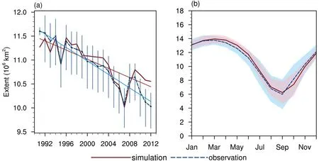
Fig. 1. Time series of the (a) annual mean and (b) seasonal cycle of monthly mean Arctic sea-ice extent from model simulations (solid red line) and observations (dashed blue line; vertical lines indicate the ranges of observations from different algorithms) over the period 1991-2012. Shading in (b) represents the range of ± 2 standard deviations.

On the other hand, it can be inferred that the variation in the variance comes from the variation in the difference between the standard deviations of the simulation and observation [Eq. (2)]. To simplify the quantification of the variance, Fig. 2d compares the temporal evolution of the standard deviations of the simulations ( s) and observations ( s).It is noteworthy that the difference between sand sobviously increases from 2008 to 2012, which contributes to the sharp increase in RMSD during the same period. In this case, the annual standard deviation represents the amplitude of the seasonal cycle of sea-ice extent. In the satellite data record, the decline in ice extent over a single melt season after 2008 exceeds 10 million km, which is not observed before 2007. A possible reason for this is that as the ice cover thins and first-year ice prevails, larger regions become vulnerable to anomalously extreme atmospheric events (Stroeve et al., 2012a). Hence, the disagreement between the standard deviations of the simulations and observations over the period 2008-2011 depicted in Fig. 2d indicates that the model fails somewhat to capture the signals from the external forcings and reproduce the seasonal variability in the sea-ice extent. The results from the other two observations also show that the variance dominates the RMSD between the simulations and observations, and the seasonal variability in the simulations should be improved.

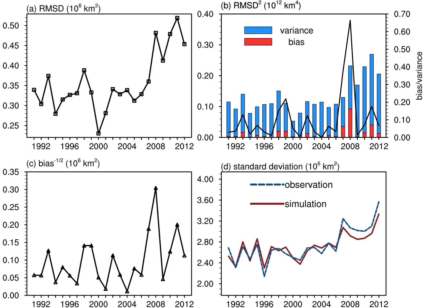
Fig. 2. Time series of the RMSD (units: 106 km2) between the detrended monthly sea-ice extent anomalies from simulations and those from observations based on the Bootstrap algorithm and the RMSD-related terms over the period 1991-2012: (a) RMSD; (b) squared RMSD (histogram), consisting of “bias” and “variance”, and the ratio of“bias” to “variance” (line); (c) absolute mean difference between simulations and observations; (d) standard deviation of simulations (red solid line) and observations (blue dashed line).

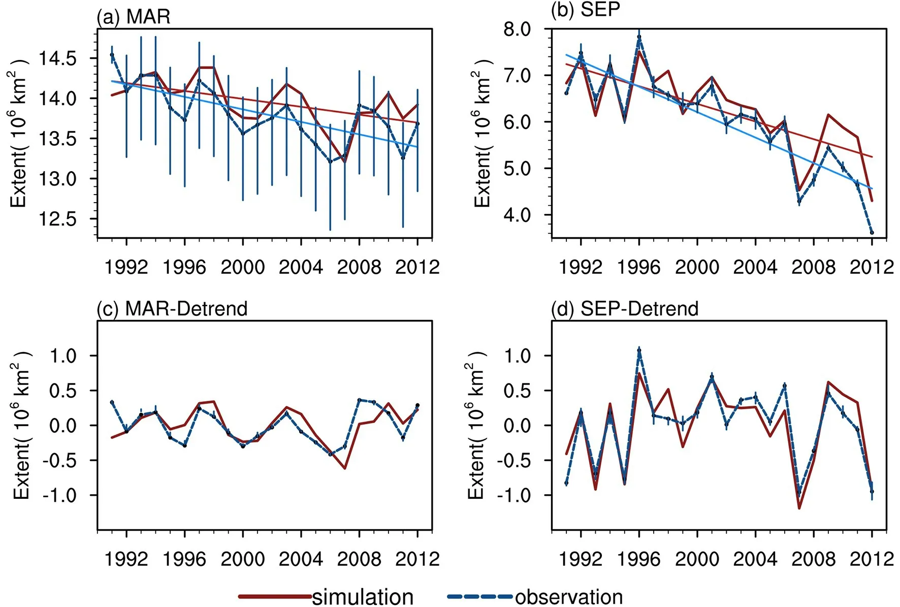
Fig. 3. Time series of monthly mean sea-ice extent in (a) March and (b) September over the period 1991-2012 and time series of detrended monthly sea-ice extent anomalies in (c) March and (d) September. Simulations are shown by the red solid line, and observations are shown by the blue dashed line. Vertical lines indicate ranges of sea-ice extent from different observations.

Therefore, it is necessary to pay attention to the variation in the representative seasons—March and September—when the sea-ice extent reaches the maximum and minimum at the end of the growth season and melt season,respectively. Thus, March and September are chosen as two representative months to explore the model’s performance under winter and summer conditions. Figure 3 shows the temporal evolution of the Arctic sea-ice extent and its linearly detrended anomalies in March and September for the period 1991-2012. The ranges of the monthly sea-ice extent from different observations are depicted in Figs. 3a and b.Although uncertainties of the sea-ice extent persist, the variability and trends in the sea-ice extent from different sources are consistent. Generally, the simulated interannual variability in ice cover is correlated well with the three observations (OBS-Bootstrap, OBS-NASA Team, and OBS-ASI),with correlation coefficients that are statistically significant at the 99% confidence level both in March and September(Table 2). The model basically overestimates the sea-ice extent in March, which contributes to a higher value of the simulated annual mean sea-ice extent, which is depicted in Fig. 1a. It is encouraging that the values of the model simulations in September are almost identical to the observations,reproducing the dramatic decrease in 2007 and the minimum in 2012. However, it is obvious that different algorithms induce higher uncertainties in determining the sea-ice extent in March; hence, most of the simulated March sea-ice extent values are within the range of different observations, while the September sea-ice extent values are not. Addi-tionally, compared with the observations, the simulated seaice extent in September is slightly overestimated after 2008,which together with the higher sea-ice extent in March can explain the increasing RMSD after 2008, as previously indicated.

Table 2. Correlation coefficients for the sea-ice extents of the simulations and observations over the period 1991-2012. The numbers in brackets are results from the detrended time series.

Table 3 lists the trends in the monthly sea-ice extent for March and September from the model simulations and observations with a 95% confidence interval. The trends in the sea-ice extent derived from different algorithms are generally compatible, and more negative trends are presented in the OBS-NASA Team and OBS-ASI than in the OBS-Bootstrap. There is a good agreement in the trend in March iceextent between simulations and the observations based on the Bootstrap algorithm. However, the rate of decline of the simulated ice extent in September of -15.2% (10 yr)±6.6% (10 yr)is significantly slower than all the three observed rates: -22.8% (10 yr)± 6.9% (10 yr), -23.3%(10 yr)± 6.6% (10 yr)and -23.6% (10 yr)± 6.7% (10 yr).The notably lower September trend in ice extent from the simulations is partly due to the overestimated ice extent after 2008, as previously indicated. Although the simulated reduction is slower than the observed reduction in both March and September, the observed trends fall within the distribution of the simulated trends at a 95% level of statistical significance. Notz (2014) found that the uncertainty arising from internal variability is the dominant reason for the differences between modeled and observed trends in sea-ice extent. Therefore, the difference between the trends of model simulations and observations is not just due to model deficiencies.

Table 3. Trends [units: % (10 yr)-1] in the sea-ice extent over the period 1991-2012 at a 95% confidence interval.

For the temporal variations of the detrended anomalies of the sea-ice extent, Figs. 3c and d show that the model is very capable of reproducing the internal variability in the ice cover in both March and September over the period 1991-2012. After detrending, the simulations and observations still maintain high correlation coefficients of averages of 0.75 and 0.90 for March and September, respectively,that are statistically significant at the 99% confidence level(Table 2). Obviously, the model performs better in simulating the sea-ice extent in September, with a higher correlation coefficient. To examine the performance of the model in more detail, we further evaluate the spatial distribution of the sea-ice concentration and its trend to investigate the discrepancies between the simulation and observation related to the location.

3.2. Spatial distribution of sea-ice concentration

To gain additional insight into the spatial discrepancies between the simulations and observations, we explore the spatial distribution in terms of the trends and RMSD in the seaice concentration for March and September. Figure 4 shows a comparison of the spatial distributions of the trends in the sea-ice concentration in units of percent per decade at each grid cell in March and September; least squares regression is used to calculate the trend in ice concentration for that month over the entire time series at each grid cell. Figures 4ac show the trend maps in March over the period 1991-2012 from the observations and simulations and the differences between them. Obviously, the sea-ice concentration in the Arctic basin is usually close to 100% in wintertime; hence,the significant trends in the sea-ice concentration in March only appear close to the ice edges in both the simulations and observations, which are observed to be negative (reduction) in the Barents Sea and Labrador Sea and positive (augment) in the Bering Sea. Furthermore, the difference between the trends of the simulations and observations is mainly positive (i.e., the downward trends in the simulation are slower than those in the observation) at the ice edges,indicating that MITgcm slightly underestimates the rate of decline of sea-ice concentration in March by less than 20%(10 yr). However, the trend maps in March are virtually identical, and the difference map shows only very minor differences near the ice edges.

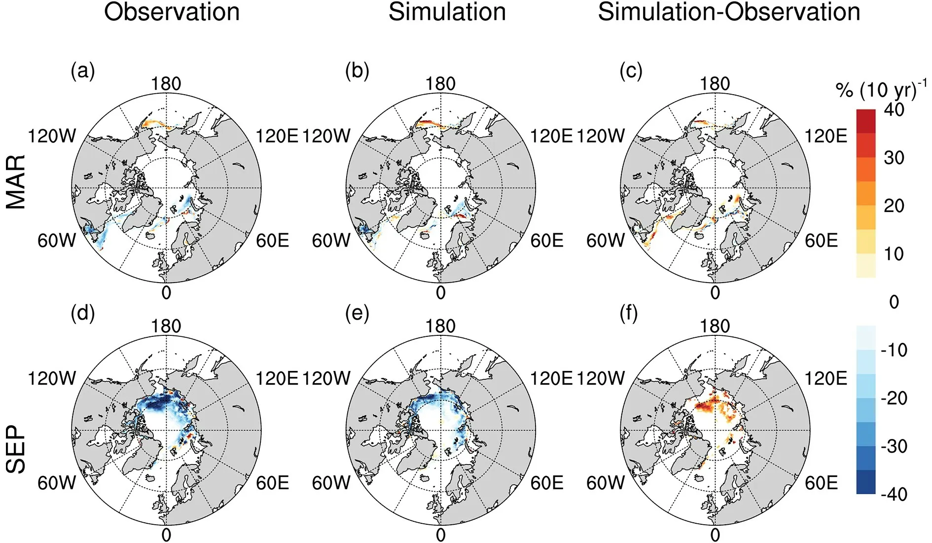
Fig. 4. Spatial distributions of the linear trends of sea-ice concentration in March over the period 1991-2012 from (a)observations, (b) simulations and (c) their difference: simulations minus observations. (d-f) As in (a-c) but for September.

Figures 4d-f compare the corresponding trend maps of sea-ice concentration in September. The trend maps of the simulations and observations show similar spatial distributions with downward trends around the eastern edges of the Arctic pack, with the most negative trends occurring in the Beaufort Sea region, where sea ice is retreating at the fastest rate in decades. The disagreements in the trend maps in the ice concentration are qualified in Fig. 4f, with the largest magnitude of difference in the Beaufort Sea, where the simulated sea ice declines at a much lower rate than the observed trend in September. The difference maps of the trends in March and September are consistent with the aforementioned discussion about the sea-ice extent trend in Table 3 stating that the rate of decline for the observed sea ice is much faster than that simulated in September.

To further assess the model performance in simulating the sea-ice concentration, Fig. 5a shows the spatial distribution of the mean sea-ice concentration from simulations over the period 1991-2012 in March. The discrepancies between the simulations and averaged observations from different algorithms are quantified by calculating the RMSD at each grid over the entire period and are shown in Fig. 5b.The large-scale features of the observed spatial distribution of the sea ice are simulated well in March, with 100% ice coverage in the Arctic basin. Both the simulated and observed sea-ice concentrations have very similar spatial distributions. except for some regional discrepancies in the Greenland Sea, Barents Sea and Labrador Sea. By checking the values of simulations minus the observations (figure not shown), we found that the model tends to overestimate the sea-ice concentration around ice edges that should be open water in March. These biases in the simulations lead to a relatively higher sea-ice extent in March, as depicted in Fig. 3a.

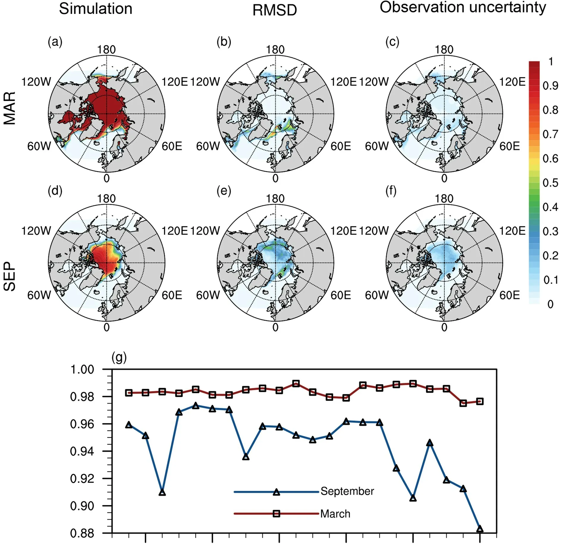
Fig. 5. Spatial distribution of the mean sea-ice concentration in March over the period 1991-2012 from (a) simulations, (b)RMSD between simulations and observations, and (c) observation uncertainty. (d-f) As in (a-c) but in September. The time series of (g) is the pattern correlation between the simulated sea-ice concentration and the observed sea-ice concentration in March (red line with squares) and in September (blue line with triangles) over the entire period.

The corresponding analysis of the spatial distribution of the sea-ice concentration in September is illustrated in Figs.5d-f. Generally, the maps of the simulations (Fig. 5d) and observations (not shown) show very similar representations of the sea-ice coverage in September but disagree regarding the ice-concentration distributions, which indicate that the model obviously overrates the ice ablation and simulates sea-ice concentrations that are low in the marginal regions.The RMSD map (Fig. 5e) indicates that there are smallvalue but large-area differences between the sea-ice concentration of the simulations and observations in September over the marginal seas of the Arctic Ocean, including the Beaufort Sea, Chukchi Sea, East Siberian Sea, Laptev Sea,Kara and Barents Sea. It makes sense that the model generally performs better in reproducing sea-ice coverage in March due to the consistent ice coverage in the late winter.However, in September, the sea ice at low and intermediate concentrations occupies a large marginal zone, which leads to a large uncertainty in the model simulations. Both the dynamics and thermodynamics of the model are more complicated regarding the sea-ice conditions at the marginal sea region, where sea-ice drifting and melt-pond formation are expected during the melt season.

To account for the uncertainty in the sea-ice concentration field obtained from the satellite data, the mean ranges of the sea-ice concentration in March and September from different algorithms for the same period are depicted in Figs. 5c and f. The differences between the sea-ice concentrations of different algorithms are apparent, particularly in September,and are generally less than 0.3. In September, large-area differences arise between the different satellite retrieval data over the Arctic Ocean, where low sea-ice concentrations with greater uncertainty in the passive microwave data prevail. However, in March, different satellite products provide very similar sea-ice concentration fields, except uncertainty arises around the ice edges, especially in the Bering Sea.The depictions of the RMSD contribute to estimating whether a certain difference between the simulations and observations lies within the observational uncertainty (Notz,2014). In most areas, the discrepancies between simulations and observations shown in Figs. 5b and e lie within the algorithmically based uncertainty in observations.However, there are obvious deviations that outrange the corresponding uncertainties around the ice edge at the North Atlantic in March and over large areas of the marginal seas in September, where the model performs worse, as discussed above.

Although the simulated sea-ice extents match the observations quite well in September, as previously indicated, the spatial distribution of the sea-ice concentration significantly differs from the observations. In addition, the similarity of the spatial distribution and the pattern correlations, which is a linear correlation between the sea-ice concentrations from the simulations and observations at corresponding locations on two different maps, are shown in Fig. 5g. It is apparent that the pattern correlation in September is much smaller than that in March each year, which means that the disagreement between the spatial distributions of the simulations and observations is stronger in September. The pattern correlation for September changes more drastically, which implies that it is harder to capture the ice distribution in a particular year, probably due to unusual weather conditions.

3.3. Preliminary evaluation of sea-ice thickness

In addition to the sea-ice coverage, the variation in the sea-ice thickness directly affected by thermodynamic and dynamic processes is essential for assessing the performance of numerical models. However, the observations of Arctic sea-ice thickness have been spatially sparse and temporally sporadic (Tilling et al., 2015). Therefore, the model-data comparisons of sea ice thickness have to be restricted to the specific periods and regions when and where observations are available.

The monthly sea-ice volumes are calculated by taking the product of the ice thickness excluding open water, the sea ice concentration, and the ice area. The observed sea-ice volumes from CryoSat-2 during the sea-ice growth period(October to April) from 2010 to 2012 are shown in Fig. 6a with uncertainties considering the algorithm uncertainty of the sea-ice thickness retrieval contained in the CryoSat-2 data product (Hendricks and Ricker, 2019). The results show that the model captures the strong seasonal cycle of growth and melt of the Arctic ice and reproduces the observed seasonal sea-ice volume changes from fall to spring. However, the model generally overestimates the seaice volume by an average of 2.87 × 10km, especially in the fall, and produces a slower average October-April seaice growth rate of 1.45 × 10kmper month compared with the 1.65 ± 0.55 × 10kmper month observed during the period. To further quantify the seasonal sea-ice thickness changes from fall (October-November) to spring (February-March), Figs. 6b and c show the overall sea-ice thickness frequency distributions with statistics (mean and standard deviation) from CryoSat-2 and the model, respectively.Both show distribution changes from fall with more firstyear ice to spring with more multi-year ice. The observed sea ice has a mean thickness of 1.08 m in the fall of 2011.Four months later, the overall thickness is 1.65 m, representing an increase of 0.57 m. In contrast, the increase in the simulated mean sea-ice thickness between the fall of 2011 and spring of 2012 is 0.35 m, starting with a mean of 1.66 m.This means that the model simulates a higher mean thickness of sea ice but underestimates the seasonal increases in sea-ice thickness. In addition, compared with those of the simulations, the sea-ice thickness distributions from CryoSat-2 peak sharply with lower standard deviations in both fall and spring. There is a relatively high probability for the model to simulate thicker ice in both seasons.

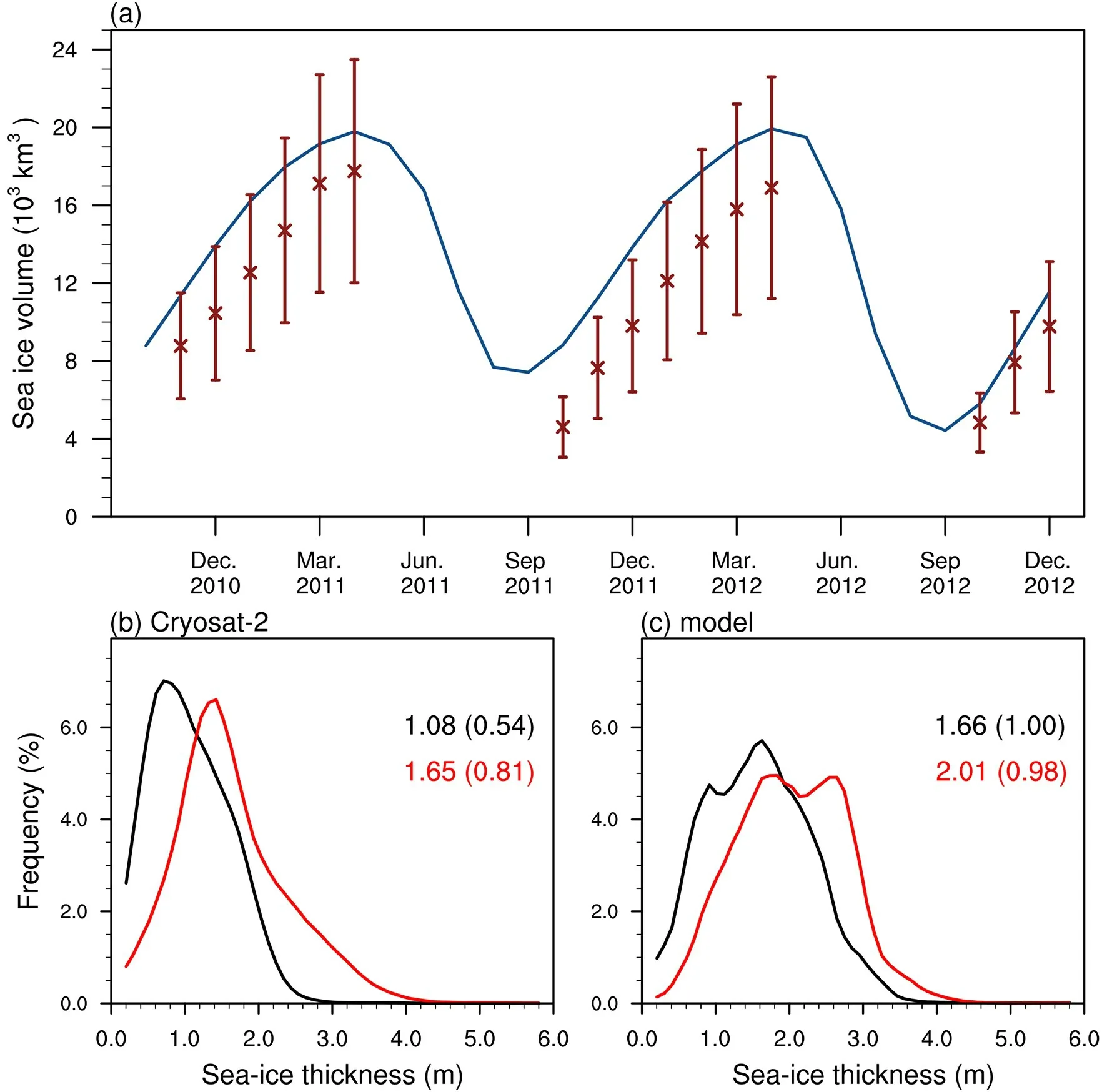
Fig. 6. (a) The Arctic sea-ice volume from Cryosat-2 (red stars) and simulations (blue line) over 2010-2012. The vertical lines indicate the uncertainties in the Cryosat-2 monthly sea-ice volume. (b) Distribution of sea-ice thickness from Cryosat-2 during the fall (black) of 2011 and the spring (red) of 2012. The numbers are the mean thickness and standard deviation (in brackets) for each distribution. (c) As in (b) but for the simulations.

To further assess the spatial differences in different seasons, the maps of the sea-ice thickness from the simulations and ICESat, and their differences, are shown in Fig. 7. The sea-ice thickness is derived from 15 ICESat campaigns that spanned a period of different days from 2003 to 2008, so the spatial distribution of mean ice thickness in spring and fall are presented. For direct comparison with the simulations, the modeled sea-ice thickness is interpolated to the ICESat grid. A combined average of February and March from the simulations is used for comparison with the ICESat spring campaigns, and the combined average of October and November is used for comparison with the ICESat fall campaigns (Schweiger et al., 2011). In general, the spatial patterns of ICESat and the simulated sea-ice thickness fields show good agreement, with high pattern correlations of 0.9 and 0.8 in spring and fall, respectively. The model tends to overestimate the thickness of the sea ice throughout the Arctic basin in spring, with a mean bias of 0.17 m. In the fall, the deviations between the sea-ice thicknesses of the model and observations are smaller, with a mean bias of-0.04 m, and the model underestimates the thickness of the sea ice around the Kara seas and the Eurasian basin. This possibly occurs because the model underestimates the advection of thick ice and the divergence between last autumn and spring (Kwok and Cunningham, 2008). In addition, the frequency distributions of the sea-ice thickness difference show that the leading difference in both spring and fall is restricted to 0-0.5 m. Additionally, Kwok et al. (2009) estimated that the ICESat thickness uncertainties are 0.5 m for individual 25-km ICESat grid cells. Therefore, it is obvious that the disagreements between the sea-ice thicknesses of simulations and observations are acceptable and the model has good performance regarding sea-ice thickness simulation. In addition, the model tends to underestimate the sea-ice thickness in the fall but overestimate the sea-ice volume, as shown above. This further demonstrates that the sea-ice concentration from the simulations is very uncertain in fall,which is consistent with the above analysis of the sea-ice concentration.

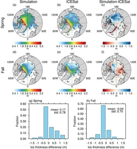
Fig. 7. Mean 2003-2008 (a, d) modeled and (b, e) ICESat sea-ice thicknesses for (a, b) spring (February-March) and (d, e)fall (October-November). The spatial distributions and the fraction distributions of the differences in ice thickness are shown in (c, f) and (g, h), respectively. The color scale is given in m.

Moreover, for a more detailed analysis of the modeled sea-ice thickness, comparisons to in-situ observations from Operation IceBridge are conducted (Sato and Inoue, 2018).These data are available in spring over the period 2009-2012 along aircraft tracks, as shown in Fig. 8a. The scatterplot (Fig. 8b) of the sea-ice thickness shows that there is a significant correlation (0.67) between the model and in-situ measurements in spring, with a mean bias of-0.06 m. Specifically, the model fails to reproduce the seaice thickness distribution in 2010, with a correlation coefficient (0.1) that is not significant at the 99% level. The mean error indicates that the model generally simulates slightly thinner ice in this region, and the RMSD (0.51) indicates that there is high uncertainty in the model regarding the reproduction of the thick ice along the coast.

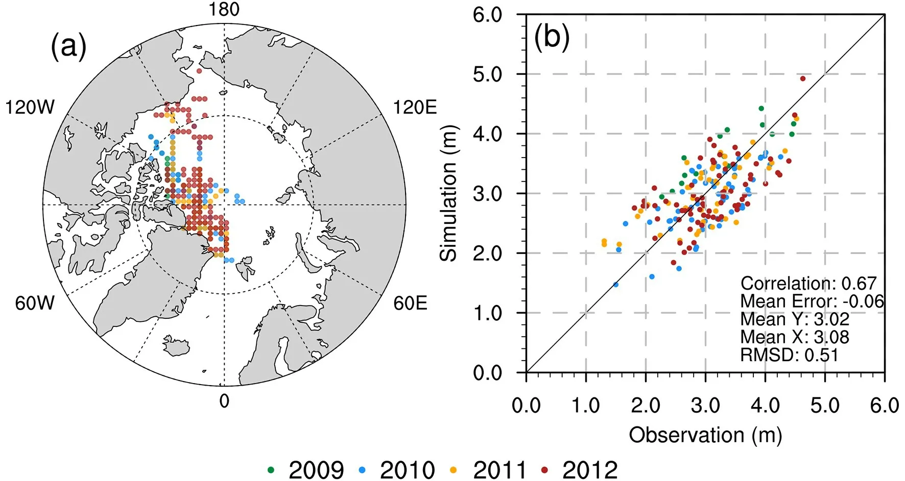
Fig. 8. (a) Locations of the observations from IceBridge in spring of 2009-2012, and (b) a scatterplot of the mean spring sea-ice thickness between observations and simulations.

In summary, the simulated sea-ice volume shows reasonable seasonal variation, and the simulated sea-ice thickness frequency distributions in the fall and spring are in good agreement with the observations. The model also reproduces spatial distributions of sea-ice thickness similar to both satellite and airborne observations. However, the model tends to present a slower growth rate for sea ice in autumn through spring. The sea-ice thickness from simulations shows different deviations due to a lack of reasonable advection. Uncertainties exist for the three observational datasets in the sea-ice extent and sea-ice concentration, but the variability and trends in the sea-ice extent and sea-ice concentration from different observational datasets are consistent.Although uncertainties exist for the three observational datasets in the sea-ice extent and sea-ice concentration, the simulations are basically within the range of observations. The trends in the sea-ice concentration and ice extent from the data derived from different algorithms are generally compatible, and the model underestimates the observed downward trends in the sea-ice extent; a comparison of the derived ice extents from different sources is presented in the Electronic Supplementary Material (ESM, Figs. S1-6). In March,disagreements between the distributions of the sea-ice concentrations of the simulations and observations only exist at the ice edges, with relatively high RMSD. Likewise, the spatial distributions of the trends in the simulated ice concentration are in reasonably good agreement with the observations in March. In September, there are generally similar spatial patterns but large-area disagreements in the ice concentration distributions over the marginal seas in the Arctic Ocean, where there is a relatively lower RMSD. Additionally, the model underestimates the downward trends in September in most of the Beaufort Sea. Apparently, the performances of the model are very different under winter and summer conditions, which indicates that different model error sources may exist that dominate in different seasons.

4. Analysis of model error sources

The disagreement in sea-ice evolution between simulation and observation is the result of a combination of many underlying factors, such as uncertainties in both the model and observation. A further explanation of the underlying causes of the difference is important for making advances in the quality of sea-ice simulations (Notz et al., 2016). As summarized by Zheng and Zhu (2008), model errors mainly result from errors in the parameterization of the physical processes, from the boundary conditions, and from errors in the numerical solution methods. For the regional ice-ocean coupled model, the variables from the atmospheric forcing and open boundaries in the ocean drive the evolution of the sea ice in a certain way. To evaluate the sources of model error that are related to the atmospheric forcing and the oceanic boundaries, the sea-ice extent is selected to evaluate the relationships between the atmospheric/oceanic forcings and the simulated sea-ice evolution and compare them with the observations.

4.1. Errors induced by atmospheric forcing variables

The net energy flux (i.e., sensible heat flux, latent heat flux, net longwave radiation, net shortwave radiation, and fraction of absorbed shortwave flux that penetrates into the ice) from the atmosphere to the ice is one of the key factors that determines the sea-ice melting at the surface, and in turn, the Arctic sea-ice cover variability reflects the changes in the atmosphere-ocean heat fluxes (Smedsrud et al.,2010). In addition, it is well known that the air temperature directly affects the growing and melting process of sea ice.Many studies have proven that gradually increasing air temperature along with shifts in atmospheric circulation correspond to sea-ice advection and lead to increasingly open water in the Arctic Ocean (Overland et al., 2008). Therefore, we investigate the relationships between the sea-ice extent and the air temperature and downward radiation, two of the most important thermal factors, to determine whether the model error is induced by the atmospheric forcing variables and whether the effects from the atmosphere in March and September are different.

As the atmospheric forcing of the sea-ice coupled model, we hope that the variation in the sea-ice cover from model simulations forced by the JRA-25 reanalysis, which is assumed to be the “true” atmospheric boundary condition,is consistent with that from observations. Therefore, the relationship between the simulated sea-ice extent from MITgcm and the atmospheric forcing variables from JRA-25 is expected to be consistent with the relationship between the observed sea-ice extent and the JRA-25 atmospheric forcing variables if the model performs perfectly. Additionally,the relationship between the observed sea-ice extent and ERA-Interim is analyzed to demonstrate the ubiquity of the expected relationship. At each grid point, the atmospheric reanalysis variables are correlated with the simulated seaice extent and the observed one in March and September over the period 1991-2012. The linear trend is removed from both time series before the correlation is computed.The linear correlation results between the sea-ice extent and the air temperature at 2 m from JRA-25 and ERA-Interim over the Arctic Ocean are displayed in Fig. 9. Figures 9a and d show the maps of the correlation between the simulated sea-ice extent and the JRA-25 2-m temperature (Simulation vs. JRA). The spatial distributions of correlations between observed sea-ice extent and atmospheric reanalysis JRA-25 (Observation vs. JRA) or ERA-Interim (Observation vs. ERA) are also shown in Fig. 9. The correlations either from the JRA-25 or from ERA-Interim show the same distributions of positive and negative centers but with different intensities, which means that the correlation coefficients can represent how the observed sea-ice extent responds to the atmospheric forcings at large scales by particular mechanisms. Furthermore, the disagreements between“Observation vs. JRA” and “Observation vs. ERA” show that atmospheric uncertainty influences the evolution of the sea-ice cover (Yang et al., 2016).

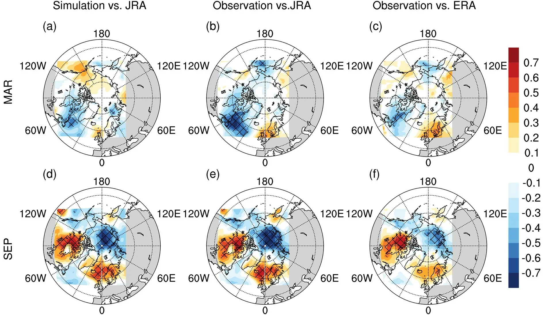
Fig. 9. Correlations between standardized sea-ice extent anomalies from (a, d) simulations or (b, e) observations, and the standardized 2-m atmospheric temperature anomalies from JRA-25 in (a, b) March and (d, e) September. (c, f) As in (b, e)but for the 2-m atmospheric temperature from ERA-Interim. Hatching covers areas that are statistically significant at the 95% confidence level. The color bar is unitless (standardized correlation coefficient).

More specifically, we find that in September, statistically significant correlations between the observed sea-ice extent and the reanalyzed air temperature at 2 m are negative over the Arctic basin, which is consistent with the physical expectation that lower air temperature leads to more extensive sea ice, and vice versa. Additionally, the air temperature at 2 m and the sea-ice extent exhibit a positive correlation in the Greenland-Iceland-Norwegian seas and northern Canada, which corresponds to the Arctic Oscillation(AO) atmospheric circulation pattern. During the AO positive phase, the surface pressure is low in the polar region,which results in a strong and consistent westerly jet at the mid-high latitudes and keeps the cold Arctic air locked in the polar region. Conversely, the belt of winds becomes distorted in the negative phase of the AO, which allows a southward penetration of colder Arctic air into the midlatitudes.Therefore, the circulation pattern produces thermal effects from the Arctic basin that are opposite to those from the surrounding regions, which further affects the sea-ice distributions in September. In March, since the Arctic Ocean is fully covered by ice, the sea-ice extent is only sensitive to the air temperature around the ice edge according to the significant correlation in Fig. 9b; this finding is consistent with the physical expectations. Through a comparison of the correlation results of March and September, we find that the model reproduces patterns similar to those of observations but exhibits different degrees of correlation with observations. Specifically, in September, the significant correlation intensity and location and spatial distributions from “Simulation vs. JRA” all match well with those of “Observation vs.JRA”, as shown in Figs. 9d and e. This also indicates that the model has a good ability to incorporate the information of atmospheric temperature into the evolution of the sea ice in September. However, in March, the model apparently underestimates or even misses the negative correlation between the sea-ice extent and air temperature around the Labrador Sea and Bering Sea. Under winter conditions, the model fails to reflect the variability in air temperatures,which may induce significant disagreements in the sea-ice concentration at the ice edges, as shown in Fig. 5c. Therefore, the model errors induced by the atmospheric temperature are more prominent in March than in September.

Sandø et al. (2010) assessed the important influence of atmospheric fluxes and found that the variability and mean value of the non-solar heat flux are considerably larger than those of the solar heat flux and that the non-solar component dominates the net heat flux. At the same time, Fig. 10 displays a result similar to that in Fig. 9, with the exception of the downward longwave radiation. Again, the correlation maps from “Observation vs. JRA” and “Observation vs.ERA” show similar patterns. Physically, downward longwave radiation exerts thermal effects on the growth and melting of sea ice similar to those of air temperatures. Likewise,despite the slight differences, the model reproduces a correlation distribution similar to that of “Observation vs. JRA” in September. Figures 10d and e show significant negative correlations over the Arctic basin and Alaska. However, in March, the model underestimates the significant negative correlations between the sea-ice extent and downward longwave radiation, as shown by comparing Figs. 10a and b;this underestimation could also be responsible for the deviations in the simulated sea-ice concentration in both the North Atlantic and North Pacific.

In addition to the thermal effects from the air temperature and longwave radiation, the evolution of the sea-ice extent is significantly affected by the momentum flux. The wind not only influences the sensible heat and the latent heat between air and ice but also directly drives the surface circulation of the ocean and ice cover, causing ridging and rafting of ice within the pack. For example, Serreze and Barry (1988) observed that geostrophic wind accounted for 60%-80% of the variance in sea-ice drift during the same year in the Arctic Ocean. The correlation distributions of the sea-ice extent against the 10-m zonal wind are shown in Fig. 11. As shown in both Figs. 11e and f, in September, a stronger westerly wind in the Beaufort Sea (i.e., the weaker Beaufort high) leads to more extensive sea ice, and vice versa. In addition, the westerly winds over Canada have the opposite impact, as indicated by the strong negative correlation. Therefore, the model can reproduce the physical relationship between the zonal wind and sea-ice extent in September, as shown in Fig. 11d. However, in March, the observed large-scale positive correlation regions between the ice extent and zonal wind (Figs. 11b and c) weaken in the North Atlantic and disappear in the North Pacific in the simulations (Fig. 11a), which indicates that the model fails to capture the impacts of the wind in March. Therefore, the model errors induced by neglecting the influence of winds over the North Atlantic and North Pacific in March could lead to uncertainties at the edge of the simulated sea ice.

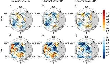
Fig. 10. As in Fig. 9 but for the downward longwave radiation.

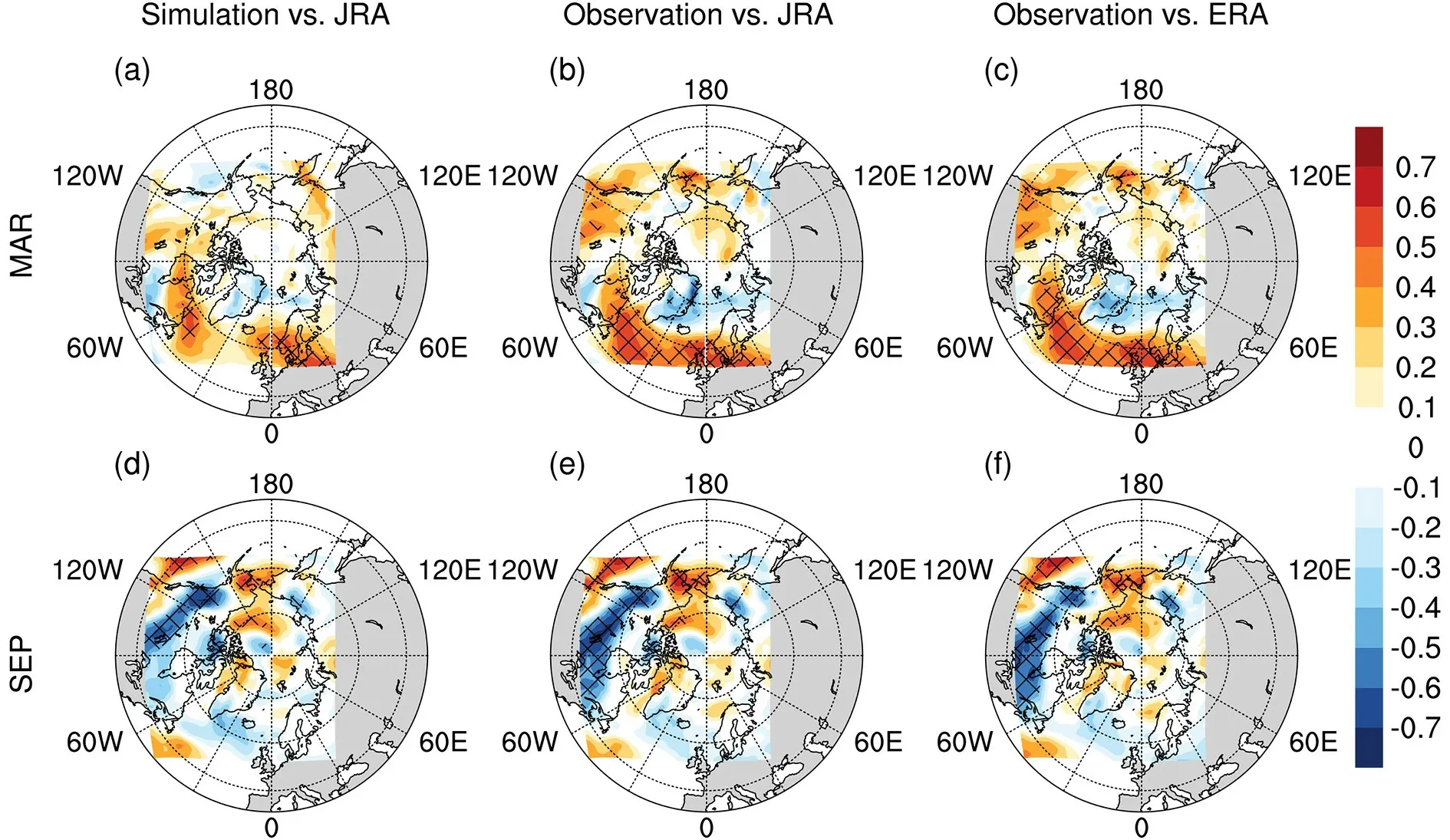
Fig. 11. As in Fig. 9 but for the zonal wind at 10 m.

For the other atmospheric forcing factors, including the 2-m specific humidity, the 10-m meridional wind and the shortwave radiation, we find the same phenomenon as described above. That is, there is a similar correlation pattern in September and a dissimilar one in March between the simulations and observations. In summary, the model performs better when reproducing the sea-ice variability according to the atmospheric forcing in September but has more deficiencies in March. This finding indicates that atmospheric forcing is one of the important sources that induces the large simulation uncertainties, especially when the model has a poor response to atmospheric forcing in March.

4.2. Errors induced by the oceanic boundary

As demonstrated in previous studies (e.g., Fichefet and Gaspar, 1988; Carmack et al., 2015; Serreze et al., 2019),the ocean still has a direct impact on the changes in sea-ice mass with respect to freezing and melting processes. Additionally, poleward ocean heat transport has been shown to be important regarding the variability in the Arctic sea-ice extent (Sandø et al., 2014). In this work, the oceanic open boundaries of the model feature warm and saline water moving from the Atlantic to the Arctic Ocean. Therefore, we continue to explore the model errors induced by the effects of the ocean boundaries, including the potential temperature and salinity of the open boundaries in the Atlantic and Pacific sectors.

Considering the longer time scale of some processes in the ocean, in Fig. 12, we illustrate the correlation coefficient between sea-ice extent and earlier ocean temperature at lead times of 1-12 months for the period 1991-2012 as a function of the ocean depth and lead time. The monthly ocean temperature of the open boundaries in the Atlantic and Pacific sectors is averaged at each level of the model.Before computation, both the sea-ice extent and ocean temperature time series are linearly detrended. Then, the correlation results are plotted for the upper 1000 m (30 levels) of the ocean, including the mixed layer and thermocline. The distributions of correlation between the observed sea-ice extent and ocean temperature of the open boundaries are referred as “Observation vs. Oceanic boundaries”, and the results from the simulated sea ice extent are referred as “Simulation vs. Oceanic boundaries” in Fig. 12. The positive and negative correlations suggest that the sea ice does respond to the ocean temperature from the open boundaries in a certain way with a delay of several months. Physically, the upper-ocean temperatures and ice extents are expected to negatively covary, since a colder ocean temperature leads to more extensive sea ice, and vice versa. In March, Fig. 12a suggests that the positive ocean temperature anomalies in the upper layer of the previous summer (i.e., ocean has an 8-month lead to ice) are followed by a relatively lower March sea-ice extent. This result is consistent with Bushuk et al.(2017), who stated that the summer subsurface ocean temperature anomalies have the potential to impact the sea-ice growth rates in the following winter. With the mixed layer deepening in the subsequent fall/winter, a significant negative correlation is found approximately 100 m below the sea surface.

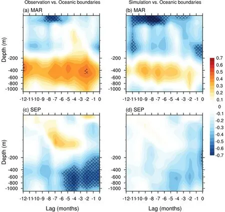
Fig. 12. Correlations between the standardized sea-ice extent anomalies from (a, c) observations or (b, d)simulations, and the standardized anomalies of the ocean temperature of the ocean boundaries at ≈ 55°N in both the Atlantic and Pacific sectors in (a, b) March and (c, d) September. Hatching covers areas that are statistically significant at the 95% confidence level. Negative lags indicate the ocean temperature leading the sea-ice extent. The color bar is unitless (standardized correlation coefficient).

In September, the sea-ice extent is significantly correlated with the ocean temperature of the thermocline with a lead time of up to 5 months, and the heat of the thermocline can influence the extent of sea ice with a shallowing mixed layer from winter to summer. Generally, the correlation patterns from simulations show reasonable agreement with those from observations in March, but the higher correlation coefficients from simulations show that the model overestimates the degree of statistical significance between leading ocean temperatures and sea-ice extents. Additionally, in September, it is obvious that the model underestimates the effects of leading ocean temperatures, although there are similar patterns. This result indicates that the sea-ice model is able to reproduce the influence from the leading surface and subsurface ocean temperatures on the March sea-ice extent but fails to reproduce the significant negative correlation between the thermocline water of the previous spring and summer and the sea-ice extent in September. Therefore, in September, the model fails to reasonably incorporate the sea temperature into the evolution of the sea ice, which is the main source of uncertainty in the simulated sea-ice extent.

Salinity plays a more important role than temperature regarding ocean density in cold polar regions. The leading correlations between salinity from oceanic boundaries within the upper 30 levels and the sea-ice extent in simulations and observations are compared in Fig. 13. In March, the sea-ice extent is not significantly correlated with the leading salinity in either simulations or observations (Figs. 13a and b).In September, similar correlation patterns with significant differences in magnitude are depicted in Figs. 13c and d. The former shows consistent negative correlations, implying that saltier water is resistant to the formation of ice, which suggests that the influence of the salinity of the upper 600 m of seawater is strong for up to 12 months prior to the observed September ice cover. However, the simulated sea-ice extents in September are not significantly correlated with the salinity at all lead times. This result indicates possible model errors from the inadequate ability of the model to capture the response of the ice cover in September to fluctuations in ocean salinity. For the ocean currents in the open boundaries, we find the same phenomenon as described above.

In conclusion, the coupled ice-ocean model is reliable due to its ability to capture the important underlying exchange processes involved in the air-ice and sea-ice interface through their physical and numerical formulations. The magnitude of the correlations between the sea-ice extent and forcing preliminarily indicates the degree of influence from the atmosphere and ocean. By examining whether the model simulations and observations yield similar significant correlation results, we find that the inherent uncertainties in the model configuration related to incorporating atmospheric forcing and oceanic boundaries, could induce the simulation uncertainties. According to the model’s performance in the simulation of the trends and distributions of sea-ice cover,the features of the disagreements between the simulations and observations in March and September are different. Additionally, the correlation analyses indicate that the model underestimates the atmospheric influence on the sea-ice evolution in March and the ocean boundaries’ influence on the sea-ice evolution in September. From these seasonal changes in the simulation uncertainties and the associated seasonal changes in the ability of the model to reflect the effects of atmospheric and oceanic forcings, we suppose that the main sources of model error are different in March and September. For example, in March, the heat and momentum fluxes from the atmosphere are not perfectly considered in the model, which influences the thermodynamics and dynamics of the sea-ice evolution. Hence, the correlations between the simulated sea-ice extent and atmospheric forcing are underestimated in March, indicating that the model underestimates the response to atmospheric forcing.In September, the model error mainly comes from the underestimation of the correlation between the ocean boundaries and sea-ice variations, which results in the aforementioned disparate behaviors between the model and the observations.

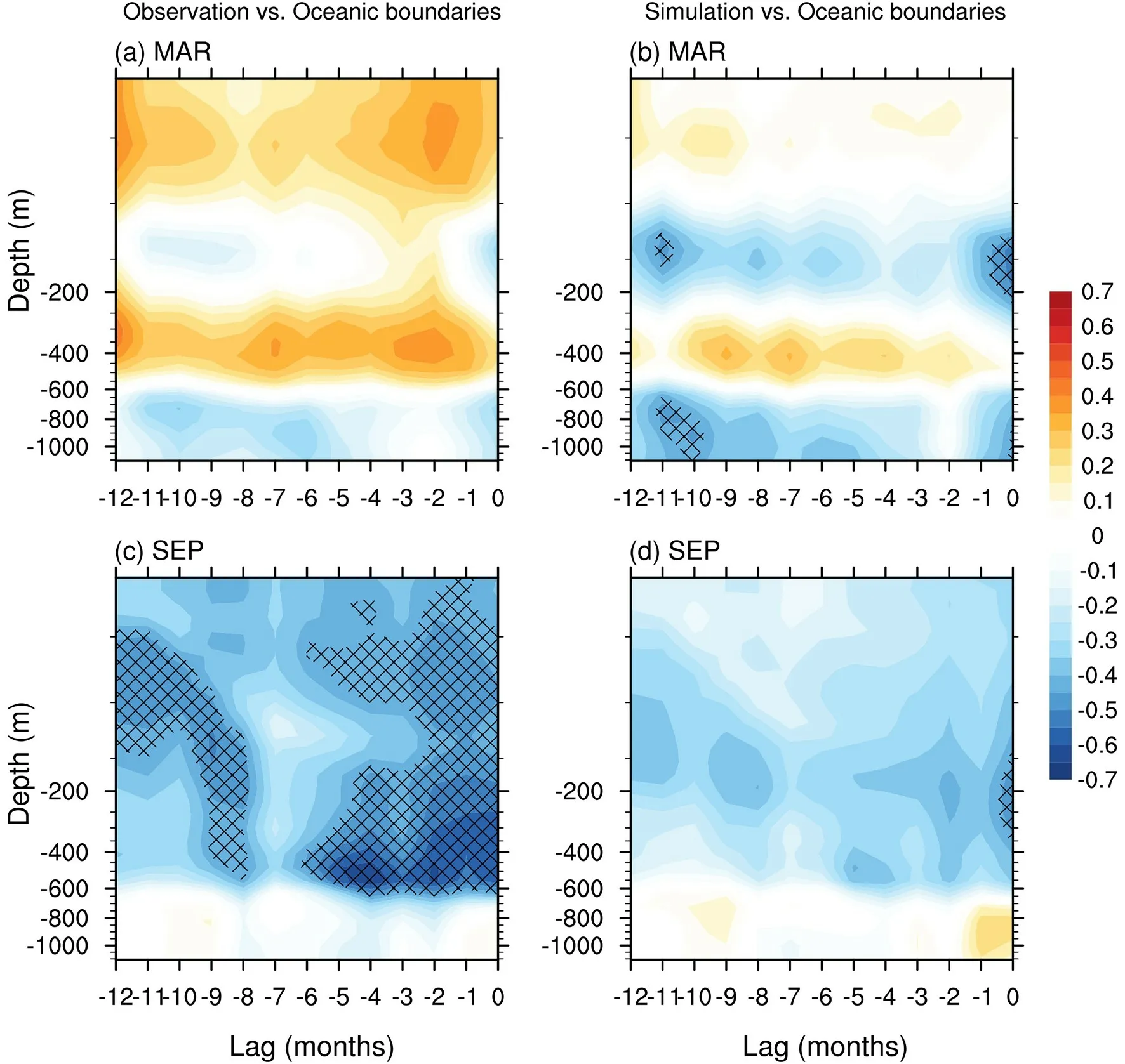
Fig. 13. As in Fig. 12 but for salinity.

5. Summary and conclusions

The dramatic changes in Arctic sea ice have gained more attention recently, and more importance has been attached to models that can provide a reasonable simulation of sea ice. In this paper, the observations of sea-ice concentration derived by different algorithms and sea-ice thickness are compared; we present the results of Arctic sea ice simulated by a regional coupled ice-ocean model based on MITgcm over the period 1991-2012, with the goal of evaluating the spatiotemporal variability and trends in Arctic sea ice. We further investigate the possible sources of the model error from the atmospheric and oceanic boundaries. Overall,there is good agreement in the seasonal-to-interannual variability in the sea-ice extent and large-scale ice distributions.However, temporal and spatial analysis shows that the icecoverage simulation performance of the model in March is quite different from that in September. In March, there is good agreement between the spatial distributions of sea-ice concentration of the simulations and observations, while significant differences in the sea-ice concentration are found only around the ice edges, and the model consistently simulates a higher sea-ice extent that is within the uncertainty of the observations. Additionally, the model slightly underestimates the downward trends in the March sea ice around the southern ice edge. We also find that the model is unable to capture the influence of the atmosphere in March, which leads to uncertainties in the sea-ice simulation at the ice edge. In September, although the model simulates reasonable sea-ice extent records, there are small-value but largearea differences between the sea-ice concentrations of the simulations and observations over the marginal seas of the Arctic Ocean, and some of the differences exceed the limits of the uncertainty range of the satellite observations. Likewise,the downward trends in the sea-ice extent are underestimated significantly in September, with the simulated sea ice declining at a much lower rate around the marginal seas, especially the Beaufort Sea. The analysis of the sources of model errors shows that signals from the ocean are missed by the model in September, which leads to uncertainty in the simulations at the marginal seas with low ice concentration.

In conclusion, the uncertainty in simulated sea ice at low and intermediate concentrations occupies most of the September ice cover and the edge of the March ice cover, resulting in temporal and spatial disagreements with observations. However, it is well known that the inherent noise in sea-ice concentration retrievals is considerable (Meier and Notz, 2010). Consideration of the sea-ice concentration data based on the Bootstrap, NASA Team and ASI algorithms shows that observational uncertainty can explain some of the discrepancies between the model simulations and observations, which indicates that the aforementioned difference is acceptable to a certain degree. Furthermore, the model deficiencies from the mechanisms used to represent the effects of atmospheric forcings and oceanic boundary conditions might contribute to the simulation uncertainties in March and September. Atmospheric forcing is found to be one of the main model error sources in March, while in September,oceanic boundary conditions are the main source. This seasonal variation in the model error sources could induce different insufficiencies in the simulation in March and September. Additionally, the model underestimates the seasonal growth of the ice volume and overestimates the ice volume,especially in the fall. The model simulates thicker ice in spring and thinner ice in the fall due to a deficiency in the sea-ice advection. This also demonstrates the great uncertainty exists in the simulations of the sea-ice thickness in different seasons.

In this work, we only focus on the representation of the sea-ice extent and sea-ice thickness, while other features in the model, such as the ice drift and ice melt/growth, are important (Holland et al., 2010) to the evolution of sea ice and must be further evaluated. More importantly, both the seasonally varying model error sources from the atmosphere and the ocean and the inaccuracy in the sea ice advection found in this work can be concluded to be model deficiencies. And that can be addressed by a more comprehensive ensemble method that reflects the model uncertainties in the regional sea-ice model that should be taken into account during the forecast process to improve the simulation results. In future work, based on the uncertainty information estimated from the current 1991-2012 modeling period, we can further establish an ensemble simulation system in an independent period (e.g., 2013-2019) to evaluate the effects of model uncertainties on seasonal sea-ice simulation. In addition, a better understanding of the model uncertainties can contribute to more reliable background information for ensemble data assimilation to improve sea-ice simulations(e.g., Lisæter et al., 2003; Yang et al., 2017).

The authors wish to thank two anonymous reviewers for their very helpful comments and suggestions.This work was supported by the National Key R&D Program of China (Grant No. 2016YFC1402705) the Key Research Program of Frontier Sciences, CAS (Grant No. ZDBS-LY-DQC010), the National Natural Science Foundation of China (Grant Nos.41876012 and 41861144015), and the Strategic Priority Research Program of the Chinese Academy of Sciences (Grant No.XDB42000000)Supplementary material is available in the online version of this article at https://doi.org/10.1007/s00376-020-9223-6.