Dynamic A* path finding algorithm and 3D lidar based obstacle avoidance strategy for autonomous vehicles
2020-11-27WangXiaohua王小华MaPinWangHuaLiLi
Wang Xiaohua (王小华), Ma Pin, Wang Hua, Li Li
(*Shanghai Key Laboratory of Power Station Automation Technology, Shanghai 200444, P.R.China)(**School of Mechatronics Engineering and Automation, Shanghai University, Shanghai 200444, P.R.China)
Abstract
Key words: autonomous navigation, local obstacle avoidance, dynamic A* path finding algorithm, point cloud processing, local obstacle map
0 Introduction
Obstacle avoidance is one of the most important tasks during vehicle’s autonomous navigation. From sensor’s aspects, lidars and cameras are commonly used for this purpose. 3D muliti-line lidar has a detection range of about 100 m with 1 cm resolution, while the range for a single line 2D lidar is 3-15 m[1]. Comparatively, 3D lidar is more reliable and now adopted by a large amount of autonomous vehicles[2,3].
After obstacles are captured in 3D lidar point cloud, it is critical to process the sensor data and design a proper local obstacle free path planning algorithm. Many local path planning algorithms have been developed. Popular local path planning algorithms are mainly the artificial potential field (APF) method, the dynamic window approach (DWA), and variants of these 2 algorithms.
The APF method was proposed by Khatib[4], where the local path is planned by artificially defined virtual forces. However, local equilibrium point may occur with this algorithm, where balanced forces keep the vehicle unmovable. In order to solve this problem, Gilbert and Johnson[5]added a special state constraint using distance functions. To apply APF method on a wheeled mobile robot, a new method based on fuzzy rules has been proposed by Zhu et al.[6]to solve this problem by modifying the control pattern or parameters in different situations. The DWA was proposed by Fox et al.[7]. DWA samples multiple sets of velocities in real time in the velocity(ν,ω) space. The vehicle trajectory at the next moment is then simulated according to each set of velocities. Each trajectory corresponding to each set of velocities is evaluated by an objective function. The trajectory corresponding to the highest score is then selected as its local path. Seder et al.[8]avoided moving obstacles by utilizing DWA considering their trajectory prediction. Gerkey et al.[9]directly searched the space of the feasible controls rather than that of the feasible trajectories. Application of DWA usually requires an accurate kinematic vehicle model.
Hart et al.[10]proposed A*algorithm in 1968. A*algorithm is a path finding method based on grid maps and it can avoid most of the unnecessary searches. In general, A*algorithm and its variants[11,12]are global path finding algorithms based on static occupied grid maps. Herein, a lidar based dynamic A*algorithm is proposed, which could find the local obstacle free path in real time.
A scenario is described as follows. An autonomous vehicle moves from a starting position to a target location with a preset global path and obstacles are detected and avoided using 3D lidar. A dynamic A*path finding method is employed and a local obstacle free path is generated in real time to guide the vehicle to avoid obstacles. The rest of the paper is organized as follows. Section 1 explains the scenario details. Section 2 focuses on the local path planning and explains the point cloud processing, the construction of the local occupied grid map, and the local path generation using dynamic A*algorithm. Vehicle hardware setup is then introduced and the experimental results are presented in Section 3. Finally, Section 4 concludes this paper and presents future perspectives.
1 Autonomous navigation scenarios
The vehicle’s autonomous navigation is usually composed of 2 parts: global path tracking and local obstacle avoidance. To test the proposed local obstacle avoiding dynamic A*algorithm, the global path tracking is not the concern of this paper. Therefore a global path is preset between the starting point and target position. Current positions of the vehicle are obtained in real time. And without obstacles, the vehicle is able to track the preset global path. Note that the effect of obstacle avoiding algorithm is closely connected with vehicle speeds. Usually, the higher the speed, the heavier the hardware’s calculation load, which deteriorates the algorithm effectiveness. For normal city vehicles, when an obstacle is detected in the way, its speed can be lower to an operational range. The vehicle speed during obstacle avoiding is considered as 2- 4 m/s.
Once an obstacle appears in the way of the global path and is within the 3D lidar detecting range, its information would be in the point cloud data outputted by the lidar. Lidar’s output is processed and the obstacle grid map is precisely calculated. The relative distance between the obstacle and the vehicle is confirmed. To be conservative and to increase the safety margin, the obstacle shape is properly expanded. After the obstacle free path is generated, it would be marked on the grid map. The first grid along this path is set as its current target and the tracking would be executed. This process is repeated until there are no obstacles. If there is no obstacle in the range, the vehicle tracks back to its global path. The flow chart of vehicle autonomous navigation is shown in Fig.1.

Fig.1 Autonomous navigation flow chart
2 Local obstacle avoidance
If an obstacle is detected along the vehicle’s global path by the equipped 3D lidar, the vehicle’s obstacle avoiding mode is activated. The local obstacle avoidance algorithm is composed of 4 parts: point cloud data processing, local occupied grid map construction, dynamic A*based local path planning, and vehicle states update.
2.1 Point cloud processing
Raw lidar data size is generally large, for example, about 300 kB/s for a VLP-16 lidar(Velodyne LiDAR Puck). Amount of raw sensor data is processed before applied in the obstacle avoidance algorithm. Point cloud processing is the following 3 steps.
First of all, in order to collect the information around the vehicle, the original 3D point cloud is filtered by a range filter and then a statistical outlier removal algorithm[13,14]. Secondly, in order to further relief the load on hardware, the filtered 3D point cloud is downsampled by a voxel grid filter[15,16]. At last, the processed 3D point cloud is converted to the 2D point cloud prepared for the dynamic A*path finding algorithm.
The flow chart of point cloud processing is shown in Fig.2.

Fig.2 Point cloud processing flow chart
2.1.1 Point cloud filtering
Point clouds around the vehicles are selected using a range filter. The point cloud outside the spatial range is then discarded. The practical space range in the experiments is as follows:

(1)
Point cloud data are further filtered using a statistical outlier removal algorithm. Those points that do not satisfy a specific statistical property are removed. In actual experiment, the statistical property is the average distance in a neighborhood. Points that deviate too much from the distance average are removed. The number of neighbors used for the average computation can be chosen by the users.
2.1.2 Point cloud downsampling
The downsampling algorithm is used to further reduce the amount of the 3D point cloud. Through downsampling, the density of the 3D point cloud is decreased while the main 3D point cloud shape is kept.
In experiments, the voxel grid filter is used as the downsampling algorithm. Voxel grid filter algorithm partitions the 3D point cloud into voxels, i.e. subclouds, or a 3D grid as is named. All of the points contained in each voxel are replaced with the centroid of that subcloud. The size of each voxel can be specified by the users. Once the size of a voxel is specified, the density of the 3D point cloud is determined.
2.1.3 Point cloud conversion
In order to design the A*algorithm, 3D lidar data are to be presented on a 2DXOYplane for the vehicle obstacle avoidance. A conversion method specified as follows.
Firstly, 3D point cloud is projected to a 2DXOYplane by setting the height valuezof the 3D point cloud to zero. Secondly, a central angleφof each point in the point cloud is calculated as follow formulas:
(2)


Fig.3 Point cloud 2D processing
In Fig.3, the 2DXOYplane is divided into 360/ρsectorial regions. The circular dots and triangle dots represent the points of the point cloud in 2DXOYplane. They are assigned to the corresponding sectorial region according to their central angleφ. The triangle dots are the closest points to the origin in each sectorial region. Therefore, they are retained while the circular dots are discarded.
In actual experiments, 0.2 ° is selected as the value ofρsince 0.2 ° is the angle resolution of the VLP-16 lidar used. The 2DXOYplane is divided into 1 800 sectorial regions. So there are maximum 1 800 points in each processed point cloud. As a result, the significant information is captured and the amount of the points of the cloud is reduced through the series of processing.
2.2 Local obstacle map construction
The next step is to create a local obstacle map based on the obtained 2D point cloud. The local obstacle map is essentially an occupied grid map, and is mathematically represented by a 2D binary matrix.
Fig.4 illustrates a local obstacle map, where the occupied grid map with a matrix size of 5×5 is shown as an example. A 5 m×5 m area is represented by this matrix and its grid resolution is 1 m. The parameters here are adjustable according to different road scenarios.

Fig.4 Illustration of local obstacle map construction
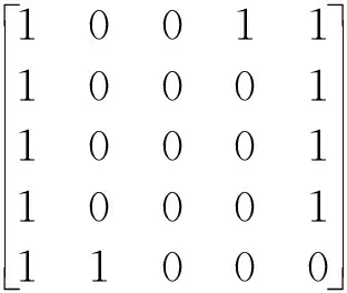
In Fig.4,Xmax,Xmin,YmaxandYminare the boundaries of the occupied grid map. Note thatXminandYminare on the negative half of the coordinate axis, and thus have negative values. The row values and column values of the grid map are represented by the index numbers on the left and the top of the grid map, respectively. The black dots represent the points of the obtained 2D point cloud. Whenever there is an obstacle detected, the number in the corresponding grid is set to ‘1’, as seen in the Fig.4 (denoted by the black dots). The value of the grid without obstacles (without black dots) is set to ‘0’. And the corresponding 2D binary matrix is as follows. This matrix is not practically produced, just for explanation.

(3)
From this 2D binary matrix, the real position (xandycoordinates) of a point in the grid map can be retrieved, and so is the real distance range of the obstacle.MxandMyrepresent the size of the grid map. The value ofMxandMyis 5 in this example.xresandyresrepresent the side length of the grid, i.e. the resolution of the grid map. The resolution is calculated by
(4)
Note that the size and the resolution of the grid map are adjustable according to the actual scene. The higher the resolution is, the larger the size of grid map matrix is. The origin of the grid map in the 2DXOYcoordinate can also be adjusted.
2.3 Dynamic A* path finding algorithm based local obstacle avoidance
Dynamic A*algorithm is used as the online local path planning algorithm for obstacle avoidance. The implementation of the obstacle avoidance process is mainly divided into the following 3 steps.
2.3.1 Obstacle area expansion
Once an obstacle is detected and the obstacle map is built as stated, the obstacle area is expanded considering the safety and kinematics of the vehicle. The expansion width and length is set by the safe distance between the vehicle and the obstacle considering the vehicle size. The expansion shape is chosen to smooth the planned local path. The expansion method shown in Fig.5 is then selected.

Fig.5 Obstacle area expansion
As shown in Fig.5, the obstacle area expansion is realized by assigning ‘1 s’ around the existing ‘1 s’ in the occupied grid. In Fig.5, the small square box in the right figure represents the original obstacle area, and the interior two pentagon boxes represent the result of the expansion of the original obstacle area. The outermost box represents the overlapped obstacle expansion area. The obstacle’s expanded size and shape can be adjusted according to the user needs. For example, if the length of the vehicle is equivalent to the length of the 3 grids and the width is equivalent to the width of the 2 grids, then the grids of the outermost circle of the pentagon box boxed expansion area in Fig.5 are removed. The experiment can be carried out with the shape and size of the adjusted obstacle expansion area.
2.3.2 Setting of the starting point and end point of the A*path planning algorithm
The starting point of dynamic A*path planning algorithm is set at the location of the vehicle. And the end point is set in the traveling direction of the vehicle. In actual experiment, lidar is rigidly amounted at the top of the vehicle, so lidar location is actually the vehicle position. Lidar is at the origin of the local planeXOYcoordinate system, so the position of the vehicle in the local coordinate system is also the origin. The grid in which the lidar is located is set as the starting point of the A*path planning algorithm, namely the center grid of the occupied grid map. A grid located at a certain distance in front of the starting point is set as the end point of the A*path planning algorithm.
As long as the sampling time is short enough, the end point of the A*path planning algorithm is in front of the starting point along the travelling direction, and the vehicle will not deviate away from the global path in a fast way. This facilitates vehicle tracking back to the global path when the vehicle has avoided obstacles.
2.3.3 Real-time local path planning
The local path generated by the A*algorithm is based on the local obstacle map in real time and the planning is updated at each sampling point. After the path is planned online, the vehicle tracks the planned obstacle free path and avoids the obstacles accordingly.
3 Experiment
Experiments are performed outdoors. First of all, an obstacle is placed on its global path of the vehicle tracking. The vehicle is then tested whether it is possible to autonomously avoid obstacles based on the dynamic A*obstacle avoidance method proposed herein. Finally, the vehicle is tested whether it is able to track back to the global path when the obstacle has been avoided.
3.1 Experimental platform with hardwares and software
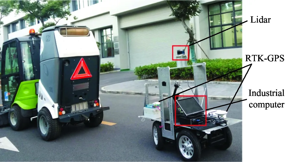
The robot operation system (ROS) is available as open source software[17]and is used as the upper control software system of the vehicle. The experiment platform (front-wheel drive four-wheeled mobile vehicle) and hardware setups are shown in Fig.6. The size of the vehicle used in the experiment is 70 cm×42 cm×155 cm. There is a 130 cm height bracket to support the lidar on the vehicle. Velodyne’s VLP-16 is used as the 3D lidar sensor in the experiment. The localization information of the vehicle is acquired by the combination of RTK-GPS (real-time kinematic global positioning system) sensor and IMU (inertial measurement unit) sensors.

Fig.6 Experiment platform and an obstacle
3.2 Local obstacle avoidance experiment
Before the experiment, a sweeper is placed on the global path of the vehicle tracking in advance to represent an obstacle, as shown in Fig.6. The vehicle tracks the planned global path when the experiment begins. Until the obstacle is detected in the obstacle detection area in front of the lidar, the vehicle enters the obstacle avoidance initial state.
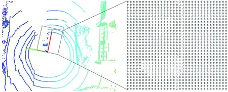
The left part of Fig.7 shows the raw 3D point cloud in the initial obstacle avoidance state, and the point cloud in the box is the detected obstacle. The right part of Fig.7 is a portion of the local obstacle map generated based on the processed 2D point cloud data in real time, which includes a local path for guiding the vehicle to avoid the obstacle. The practical local obstacle map is a lidar-centric occupied grid map, whose size is 65 m×65 m and resolution is 35 cm. In the right part of Fig.7, the number ‘1’ denotes the obstacle, ‘2’ is the starting point of the A*path finding algorithm, ‘3’ is the found local path grid, ‘4’ is the end point of the A*path finding algorithm.

Fig.7 Raw point cloud and local obstacle map of the obstacle avoidance initial state
Fig.8 shows the raw 3D point cloud information in the state where the vehicle is avoiding the obstacle and the corresponding local obstacle map containing the local path. The meaning of the contents shown in Fig.8 is the same as that of Fig.7.

Fig.8 Raw point cloud and local obstacle map of the obstacle avoidance state
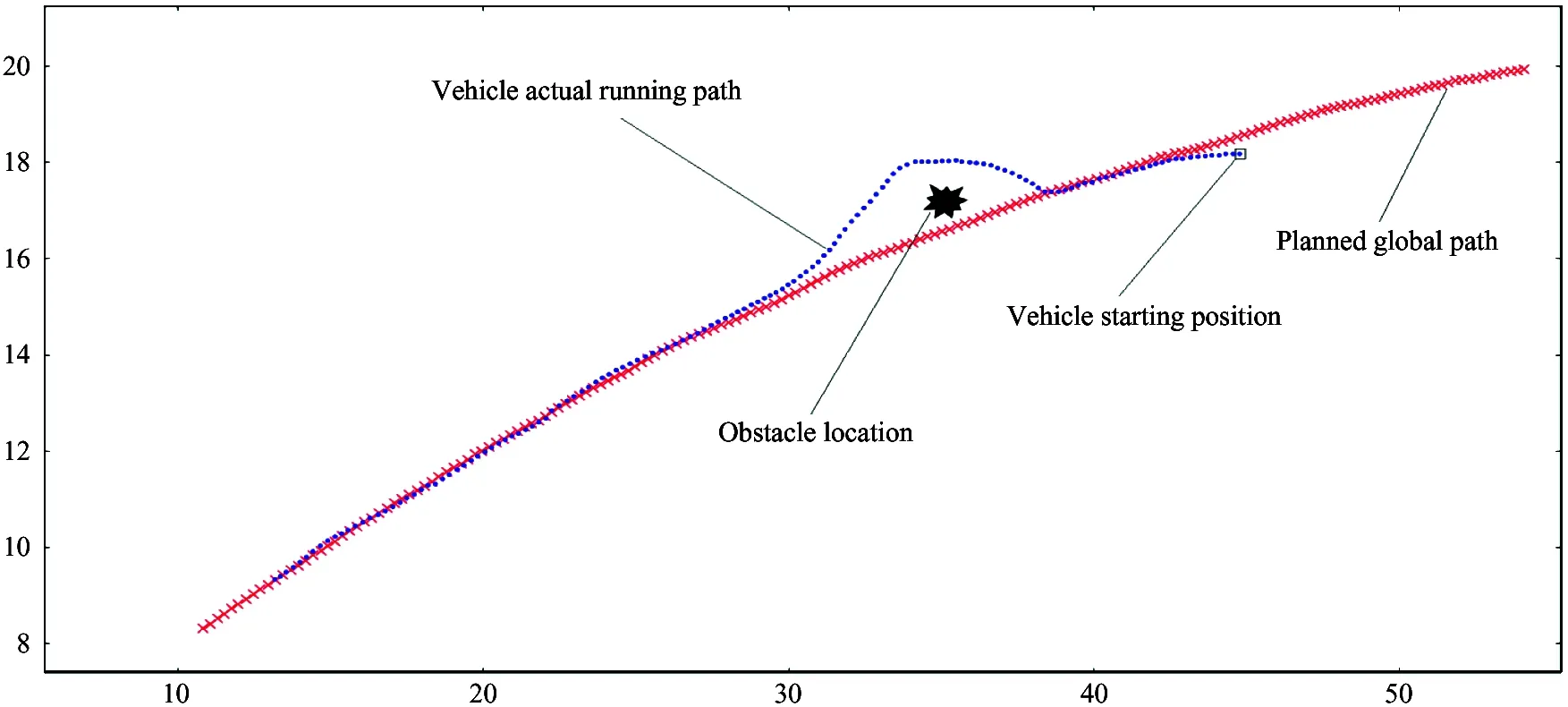
The vehicle performs local path planning for the obstacle avoidance under the guidance of a local path generated in real time. Once there is no obstacle in the lidar detecting range, the vehicle tracks back to its global path. The vehicle actual running path is obtained by recording the localization information collected by RTK-GPS. The planned global path and the obtained vehicle’s actual running path are shown in Fig.9.

Fig.9 Planned global path and actual running path
As shown in Fig.9, the global path point is represented by symbol ‘×’, the vehicle actual running path is represented by dots. Based on the comparison of the 2 paths, it can be found that the vehicle can autonomously avoid obstacles and track back to the global path.
4 Conclusions
A dynamic A*path finding algorithm based local obstacle avoidance method is proposed by this paper. A 2D local obstacle map of the 3D environment around the vehicle is constructed in real time using 3D lidar. The vehicle uses the A*algorithm to perform local path planning in real time in the constructed local obstacle map to avoid obstacles. Experiments show that the vehicle can autonomously avoid obstacles using the obstacle avoidance method, and the feasibility of this obstacle avoidance method is verified. Some limitation remains and some work still have to be done in order to be able to use this method in most of the actual scenarios. In future work, the constraints of the actual road need to be considered to prevent the vehicle from driving out of the safe driving area during the obstacle avoidance process.
杂志排行
High Technology Letters的其它文章
- Experimental study on vibration suppression in a rotor system under base excitation using an integral squeeze film damper
- Grouping pilot allocation scheme based on matching algorithm in massive MIMO system
- Fraudulent phone call recognition method based on convolutional neural network
- Behavior recognition based on the fusion of 3D-BN-VGG and LSTM network
- An effective indoor radio map construction scheme based on crowdsourced samples
- Optimal UAV deployment in downlink non-orthogonal multiple access system: a two-user case
