DYNAMIC ANALYSIS AND OPTIMAL CONTROL OF A FRACTIONAL ORDER SINGULAR LESLIE-GOWER PREY-PREDATOR MODEL∗

Linjie MA (马琳洁) Bin LIU (刘斌)†

School of Mathematics and Statistics, Huazhong University of Science and Technology,Wuhan 430074, China Hubei Key Laboratory of Engineering Modeling and Scientific Computing,Huazhong University of Science and Technology, Wuhan 430074, China

E-mail : mlj0314@126.com; binliu@mail.hust.edu.cn

Here x(t) and y(t)are the population sizes of prey and predator,respectively;E is the harvest;the parameters r and s are intrinsic growth rates of prey and predator, respectively; d is the environmental carrying capacity for the prey; a1and a2are the maximum values of the per capita reduction rate of prey and predator;n1and n2measure the environmental protection to prey and predator, respectively; q is the harvest ability coefficient; m1and m2are constants.If all the parameters are positive, we say that the model is biologically feasible.

The Leslie-Gower model (1.1) has been studied by many authors. For dynamic behavior,the global stability and existence of periodic solutions of model (1.1) were investigated in [4].[5]and[6]discussed the global dynamics of model(1.1)with stochastic perturbation. [7]mainly investigated local bifurcations of model (1.1) consisting of saddle-node and Hopf bifurcations.The local existence of a limit cycle appearing through local Hopf bifurcation and its stability were investigated in [8]. Considering the effect of control, in [9], the author incorporated an impulsive control strategy to ensure the global stability of periodic solutions for system (1.1)and derived the sufficient conditions for stability. As far as we know,few results have discussed optimal control problems for model (1.1).

In 1954, in studying of the effect of the harvest effort on the ecosystem from an economic perspective, Gordon[10]proposed an algebraic equation to investigate the economic interest of the yield of harvest effort. Naturally,differential and algebraic equations form the mathematical model of the system:

Recently, Zhang et al. established a class of differential-algebraic (singular) integer-order systems and analyzed their dynamic behaviors (see, for example, [11–14]). In [13], Zhang et al.studied the existence and stability of equilibrium points under the condition of zero economic profit and positive economic profit, and gave the sufficient conditions for the existence of bifurcations. Afterwards,in[15],the local stability analysis of a singular Leslie-Gower predator-prey bioeconomic model with time delay and stochastic fluctuations were discussed, and the impact of delay on its dynamic behavior was explored. [16]described a prey-predator fishery model,and the dynamic behaviors and the phenomenon of singularity induced bifurcation in the model system were discussed. It is worth noting that singularity induced bifurcation may lead to an impulse phenomenon in the bioeconomic model. Naturally, we hope to introduce a control variable to balance the system. In reference [13, 16], a state feedback controller was designed to eliminate the singularity induced bifurcation and impulsive behavior of the model system.Moreover,in [13], on the basis of the singularity induced bifurcation, the optimal control problem with minimizing control energy was proposed,and the local optimal controller was obtained.In [8], the optimal control problem with maximizing revenues was discussed and Pontryagin’s maximum principle was obtained to characterize the optimal singular control.

The fractional order model is an important tool to describe memory effects in prey-predator models and to investigate their more complex properties. It is well known that the differential equations with fractional order are generalizations of ordinary differential equations to non-integer order; this occurs more frequently in research areas, such as engineering, physics,electronics, biology, and control of systems ([17–21]for example). Moreover, several kinds of fractional derivatives have been introduced to investigate the fractional order systems; see for example [22–24]and reference therein.

Recently, the study of fractional order prey-predator models has received great attention.In [25], the dynamic behavior and the local stability of the equilibria were discussed for the fractional Leslie-Gower model system. In [26], the existence, uniqueness, non-negativity and boundedness of the solutions as well as the local and global asymptotic stability of the equilibrium points were studied for a fractional-order Rosenzweig-MacArthur model incorporating a prey refuge. For control problems, [27]investigated a novel incommensurate fractional-order predator-prey system with time delay and a linear delayed feedback controller was introduced to successfully control the Hopf bifurcation for such systems.

The fractional singular models are of great interest because they have many applications in fields such as electrical circuit network, robotics and economics (see for example, [28–32]). For fractional singular control models, there are many challenges and unsolved problems related to stability and so on. A fractional-order singular prey-predator model was introduced and dynamic behavior was discussed in [33]. Here the authors mainly discussed the stability of the singular system. To the best of our knowledge, few articles describe the control and optimal control problem for fractional-order singular bioeconomic models.

Being directly inspired by the above mentioned papers, we introduce the fractional order singular Leslie-Gower prey-predator model with Michaelis-Menten type prey-harvesting:

We study the solvability, stability and the bifurcation phenomenon performing to this system.For the instability point, corresponding control strategies are introduced to stabilize the system and eliminate the SIB bifurcation phenomenon. In addition, the more usual control strategies are studied in order to ensure less control energy, less total cost of harvesting, and less density of the two populations.

It is worth mentioning that our work is very different from [8, 13, 33]. First, in [8], the authors discussed the integer order model; we introduce the fractional derivative in our model and discuss a much more accurate behavior of the dynamic systems. Secondly, [33]introduced a fractional-order singular prey-predator model where the harvesting team is linear; in our model, the Michaelis-Menten type prey-harvestingis nonlinear,which is more in line with real life, though of course more complicated. Thirdly, [33]is mainly concerned with the qualitative properties of the system for the problem brought by the model itself,no method was given;in our work,we shall introduce a proper control team to stabilize the system,and we also discuss the optimal strategy. Fourthly, the cost functional in [13]only considered minimizing the control energy;we try to minimize the total cost of harvesting and control energy as well as the densely of the prey and predator, which makes the optimal control problem more general and practical.

The rest of the article is organized as follows: in Section 2,we recall the preliminaries about fractional calculus. The proposed fractional order singular bioeconomic model is introduced and the solvability is discussed in Section 3. In Section 4, the local stability and bifurcation of our system are investigated and a state feedback controller is designed to overcome the singular induced bifurcation. In Section 5, we state an optimal control problem and obtain the corresponding optimal controller. In Section 6, the numerical solutions of the fractional order singular bioeconomic model are carried out to show the feasibility and effectiveness of the obtained result. We finish by stating our conclusions in Section 7.

2 Fractional Order Integral and Derivative

In the section, we recall some basic definitions concerning the fractional calculus.

Definition 2.1(see [34]) Let f(·) be a locally integrable function in interval [a,b]. For t ∈ [a,b]and α > 0, the left and right Riemann-Liouville fractional integrals are defined,respectively, by

where Γ(·) is the Eular gamma function.

Definition 2.2(see [34]) Let f(·) ∈ ACn[a,b]and α > 0; the left and right Caputo fractional derivatives are defined, respectively, by

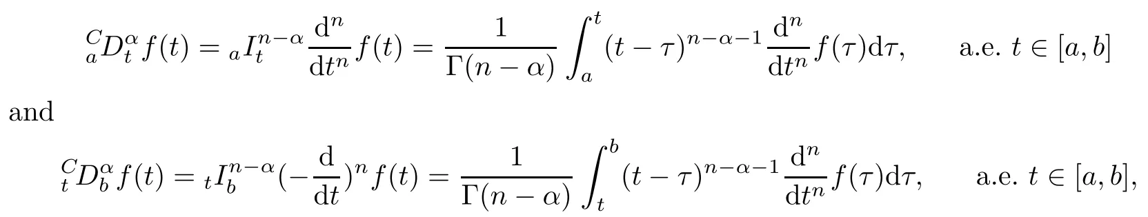
where n ∈ N is such that n − 1< α ≤ n.

Here and throughout the article, only the Caputo definition is used, because the Laplace transform allows the use of initial values of classical integer order derivatives with clear physical interpretations.

Definition 2.3Suppose that (Ξ,A) is a matrix pencil over Rn. It is said to be regular if there is some λ ∈ C such that

Lemma 2.4Suppose that (Ξ,A) is a matrix pencil over Rn. One can find nonsingular matrices P and Q such that

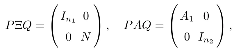
where n1+n2=n, A1∈ Rn1×n2, and N ∈ Rn1×n1is a nilpotent matrix.

Lemma 2.5(see[35]) Consider the N-dimensional fractional differential equation system

where A ∈ Rn×nand α ∈ (0,2).

(i) The solution x = 0 is asymptotically stable, if and only if all eigenvalues λj(j =1,2,··· ,N) of A satisfy

(ii) The solution x=0 is stable,if and only if all eigenvalues of A satisfyand eigenvalues withhave the same geometric multiplicity and algebraic multiplicity.

Definition 2.6(see [25]) An equilibrium point is of saddle type if the Jacobian matrix at this point has at least one eigenvalue λ1in the stable region;that is,and has at least one eigenvalue λ2in the unstable region; that is,

Definition 2.7Consider the linear fractional singular system

where x ∈ Rn, u ∈ Rmand y ∈ Rrare the state, control input and the measure output,respectively; Ξ,A ∈ Rn×n, B ∈ Rn×m, C ∈ Rr×n, Ξ is singular. And the system is said to be controllable if one can reach any state from any admissible initial state and initial control.

Lemma 2.8(i) ([36]) System (2.1) is controllable if and only if

(ii) ([37]) System (2.2) is asymptotically stable ifwhere λiare the eigenvalues of matrix A.

Lemma 2.9(see [38]) For α ∈ (0,1), system (2.1) is asymptotically stable if and only if there exist two matrices M,N ∈ Rn×nsuch that

Lemma 2.10(see [29]) For α ∈ [1,2),system(2.1)is asymptotically stable if and only if there exists a matrix P =P⊤>0 such that

3 Fractional Order Singular Leslie-Gower Prey-predator Model

In accordance with the advantages of fractional calculus, compared to the integer case as mentioned in introduction, we introduce the fractional order model by replacing the usual integer order derivatives in (1.1) by Caputo-type fractional order derivatives to obtain the fractional order system

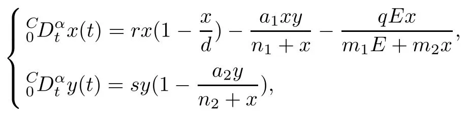
where 0 < α < 2, t ≥ 0. In fact, the fractional order system is more suitable than the integer order one in biological modeling due to the memory effects.

By the economic theory regarding the effect of the harvest effort on an ecosystem from economics, the model above can be extended. An algebraic equation of economic interest is established as follows:

Here p is the price of a unit of the harvested biomass, c is the cost of a unit of the effort, and m represents the net economic profit.

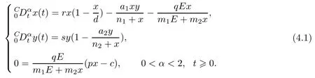
On the basis of the discussion mentioned above, the singular fractional order model of the prey-predator system, which consists of two fractional-order differential equations and one algebraic equation, can be expressed as follows:

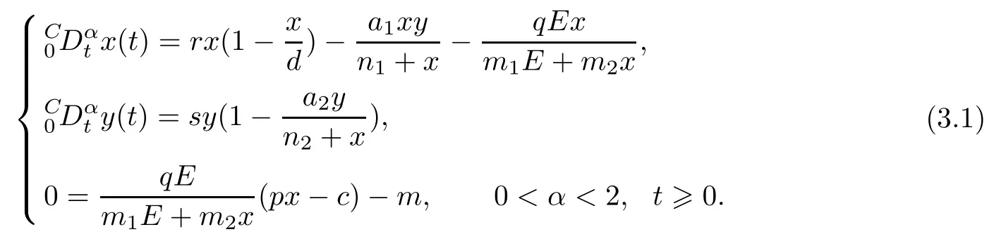
System (3.1) can also be written as

where F :R3→ R3, X(t)∈ R3and the matrix Ξ ∈ R3×3are of the following form:

In a fashion similar to [33], we establish the following solvability:

Theorem 3.1The fractional order singular model of predator-prey system (3.1) is solvable if

ProofSystem (3.1) can be linearized to the constant coefficient system

where A is the Jacobian matrix in a neighborhood of the equilibrium pointas follows:

It is adequate to calculate the determinant of the matrix λΞ − A as follows:

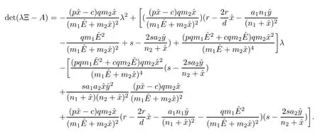
The condition of regularity is always held ([28]); that is,for some λ ∈ C(C is the field of complex number). Also, whendeg(det(λΞ −A)) = rank Ξ, in which guarantees the impulse freeness condition of the system (3.2), while at the pointAccording to the Definition 3.1 and Remark 3.1 in [39],system(3.1)is(i)always regular,and(ii)impulse free at all points exceptso the system is index one. As a result, there is no impulse behavior near the equilibrium point. By applying the implicit function theorem, system (3.1) is solvable.

4 Local Stability Analysis and Bifurcation for Model System

In this section, we mainly investigate the local stability of singular system (3.1) when the economic profit is zero; that is,

Furthermore, a state feedback controller is designed to stabilize the system at the interior equilibrium.

When m=0, the equilibrium points are the solutions of the following equations:

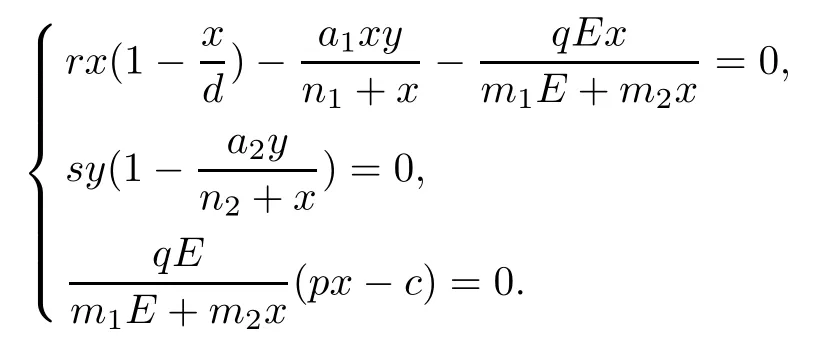
Moreover,considering that x and E cannot be zero at the same time,we have that x, y, E ≥0 and the equilibrium points are as follows:

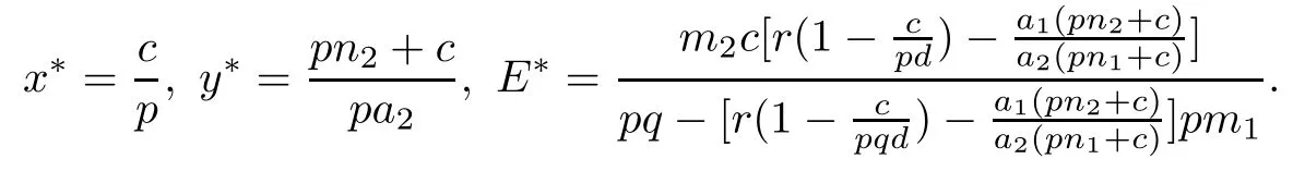
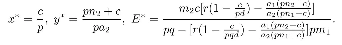
and x∗, y∗and E∗are

In what follows, the local stability of these equilibrium points is investigated.

Theorem 4.1For system (4.1),

(1) The equilibrium point P1(d,0,0) is always a saddle point;

Proof(1) The Jacobian matrix of system (4.1) evaluated at P1is

The eigenvalues of JP1are λ1= −r < 0 and λ2= s > 0. Thus,By the definition of a saddle point, the result becomes clear.

The eigenvalue of JP2is λ =s>0. Hencewhich proves (2).

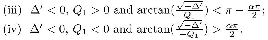
Theorem 4.3Assume that for system (4.1) there exists at least one equilibrium point,in the form ofThen, P3is locally asymptotically stable if one of the following conditions is satisfied:

(i) ∆′>0 and Q2>0;

(ii) ∆′=0 and Q1>0;

The equilibrium P4(x∗,y∗,E∗) is a singular point which may show the singularity induced bifurcation behavior.

Theorem 4.4The singular model (4.1) has a singularity induced bifurcation at the interior equilibrium, and m = 0 is a bifurcation value. Furthermore, the stability switch occurs as m increases through 0.

ProofAccording to the economic theory in [10], there is a phenomenon of bioeconomic equilibrium when the economic interest of the harvesting is zero; that is, m = 0. For model system(4.1),an interior equilibrium P4(x∗,y∗,E∗)can be obtained in the case of a phenomenon of bioeconomic equilibrium, where

Letting m be the bifurcation parameter and H(t) = (x(t),y(t))⊤, the model system (3.1) can be expressed in the semi-explicit form

(i) By simple computing, we have

This implies that dimKer(DEg(H(t),E(t),m)has a simple zero eigenvalue. In addition,

(ii) Furthermore, it can be calculated that

According to the above items,(i)–(iii),the conditions for singularity induced bifurcation,which are introduced in [40], are all satisfied, and hence model system (3.1)has a singularity induced bifurcation at the interior P4and the bifurcation value is m=0. Along the lines of the above proof, by simple computing, we have

Therefore, we have

According to Section III (A) of [40], this means that, when m increases through 0, one eigenvalue of differential algebraic model system (3.1) moves from C−to C+ along the real axis by diverging through infinity; the movement behavior of this eigenvalue influences the stability of model system (3.1).

Remark 4.5Generally speaking, the singularity induced bifurcation is due to the eigenvalues of the related fH− fEgE−1gHdiverging to infinity when the Jacobian gEis singular.Thus it is a new type of bifurcation which does not exist in an ordinary differential system.

Remark 4.6From the above theorem, we know that singularity induced bifurcation can cause the differential algebraic system to go from being stable to being unstable. From the bioeconomic perspective, this result in an impulse phenomenon,which may lead to the collapse of the proposed model system. In the prey-predator ecosystem,the impulse phenomenon of the ecosystem usually means the rapid growth of the species population, which will cause damage to the prey-predator ecosystem. Furthermore,the instability of the differential algebraic system will not be conducive to the sustainable development of harvesting on the ecosystem. Therefore, it is necessary to eliminate the impulse phenomenon caused by the singularity induced bifurcation and to stabilize the differential-algebraic model system (3.1) when the economic interest of harvesting is positive.

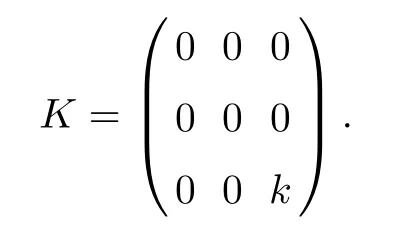
Next, we introduce the state feedback controllerwhere u(t)=kv(t), k is a net feedback gain, and v(t) is an executable input. Then, near the equilibrium point P4, we obtain the linear system

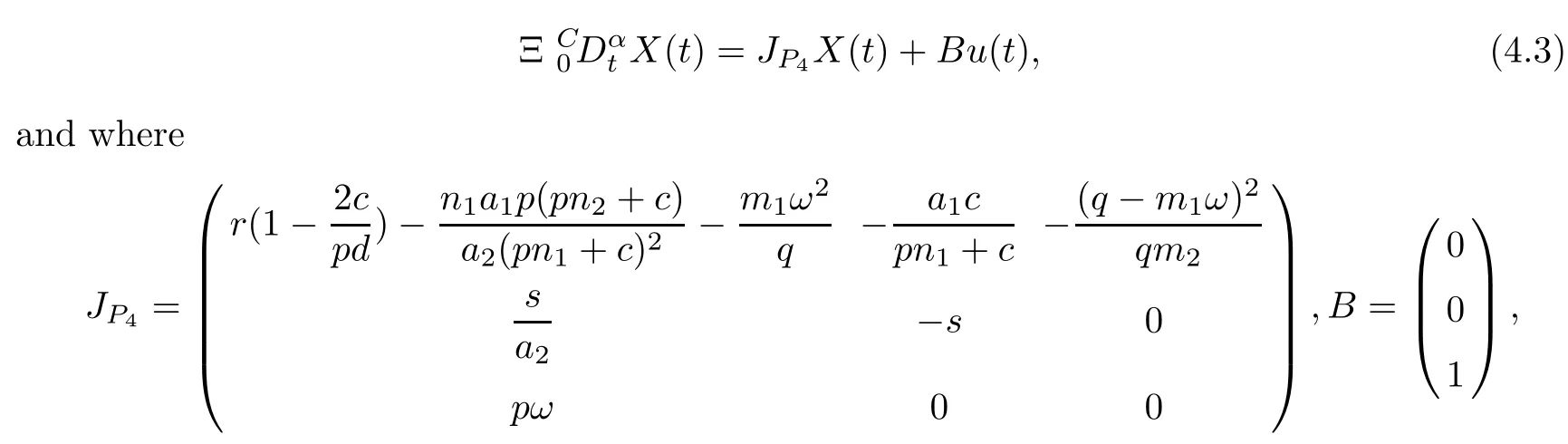
Choosing v(t)=E(t)−E∗,we rewrite system(4.1)to a new controlled differential algebraic system as follows:

Theorem 4.7The differential algebraic system (4.3) is stable at P4if

(i) for α ∈ (0,1), there exists matrix M,N ∈ R2×2such that the following holds:

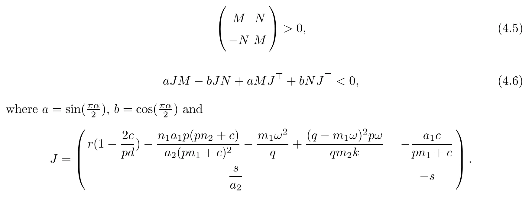
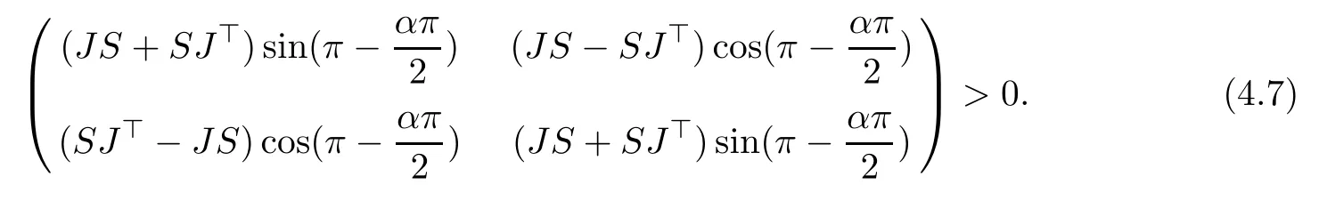
(ii) for α ∈ [1,2), there exists a matrix S =S⊤>0 such that

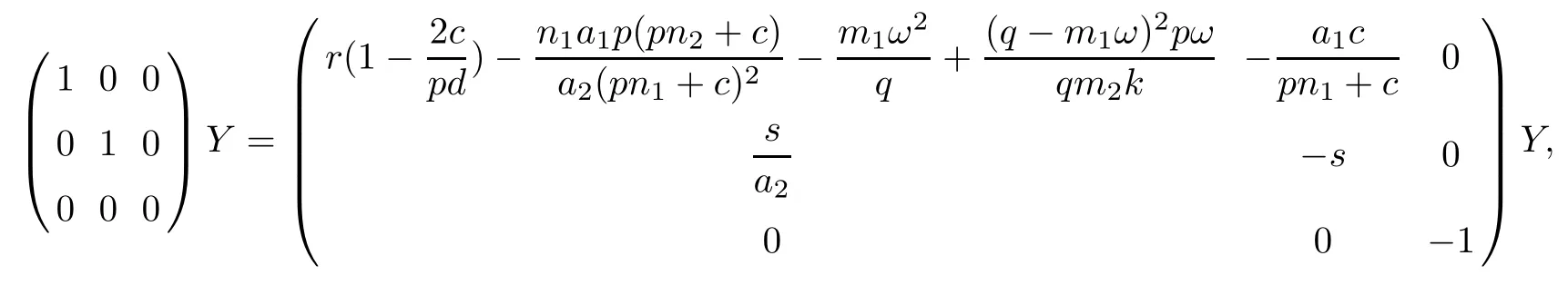
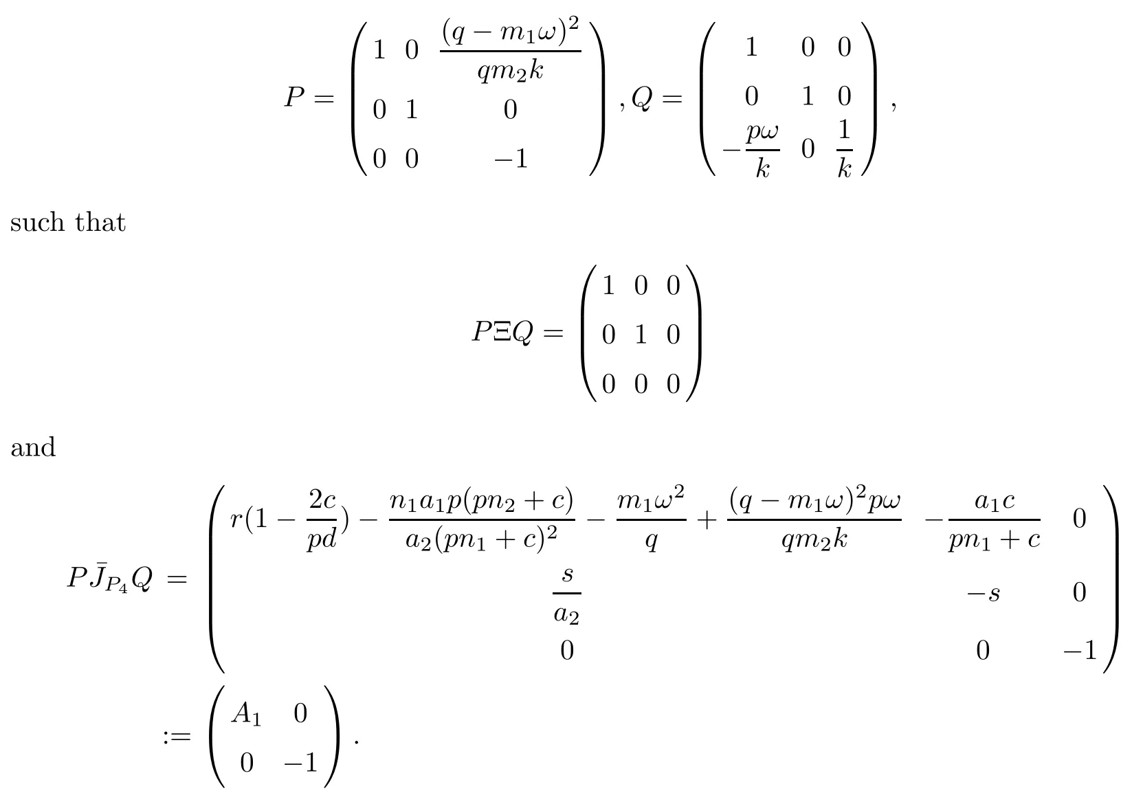
ProofDefine nonsingular maps P,Q ∈ R3×3:

That means our system can be changed into the new system:

By Lemma 2.9 and Lemma 2.10, we immediately obtain the results.

Remark 4.8From [41], we know that the Kronecker index of (3.1) is 1 if m = 0, and that it is 2 if m = 0. One idea is adding a control term to make the Kronecker index of the new system consistent with the case that m = 0. Our method is similar, but different from changing the matrix pencil {Ξ,JP4} to the Kronecker normal form. Also, we determinedly do not change the Kronecker index.

Remark 4.9Our method is very different from[29],where the authors gave sufficient conditions for the robust asymptotical stabilization with the fractional order α satisfying 0< α <2;this approach is restrictive because it involves the assumption that the system is normalizable.Thus the approach is essentially a normal system solution method instead of a sheer singular system solution method. Our main idea is to change the singular system into a stable algebraic system and a differential system. The method,however,is still the same as the singular system solution method.

Remark 4.10We design a feedback control k(E − E∗) to stabilize our model. This implies that we can adjust harvest effort to balance our ecosystem, and this brings two effects:on the one hand, we obtain the sustainable development of the prey -predator ecosystem; on the other hand,the ideal economic interest of harvesting can be obtained. It is noteworthy that these elements also make our method more consistent with real life.

5 Optimal Control for Model System

On the basis of the last section,a feedback controller is designed to eliminate the singularity induced bifurcation and stabilize the model system around the interior equilibrium P4. In this section, we hope to select an optimal controller which not only stabilizes the model system around the interior equilibrium P4, but also consumes less control energy, less total cost of harvesting, and less density of the two populations. This is an optimal control problem. In contact to last section, here we consider adding control to all three equations in general.

Consider the singular model system

where F :R3→ R3, X(t)∈ R3and the matrix Ξ ∈ R3×3are of the following forms:

where u(t)∈R3is a control input.

The energy functional is

Define the set of controls

where U is the control set. Any element in U is called a control (on [0,∞]).

A pair (x(·),u(·)) is said to be admissible if (5.1) is satisfied. The set of admissible pairs and admissible controls are defined by

Then our optimal control problem can be stated as follows:

Problem (P)Findsuch that

For convenience of calculation, we use the following transformation:

Theorem 5.1For system (5.1) with energy functional (5.2), there exists locally optimal control v(t) at the equilibrium P4(x∗,y∗,E∗):

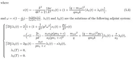
Here, x1(t) and y1(t) are the solutions of linear systems

ProofConsider the linearized system of the transformed model system around interior equilibrium P4:

Select the state feedback controller

where V(t)∈R3is the new input vector and

Substituting (5.4) into (5.3), we obtain

From Theorem 4.1, we know that there exist two nonsingular matrices,

That means under the coordinate transformation

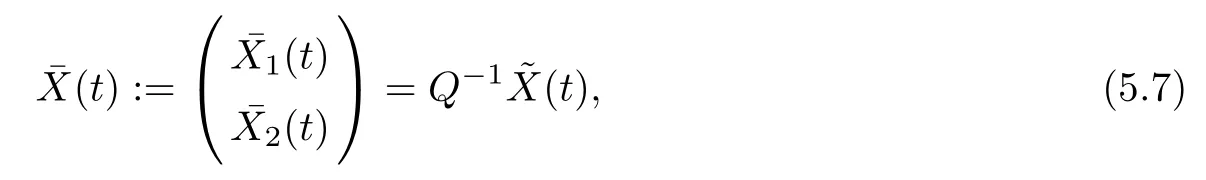
the fractional singular control system (5.5) is transformed to

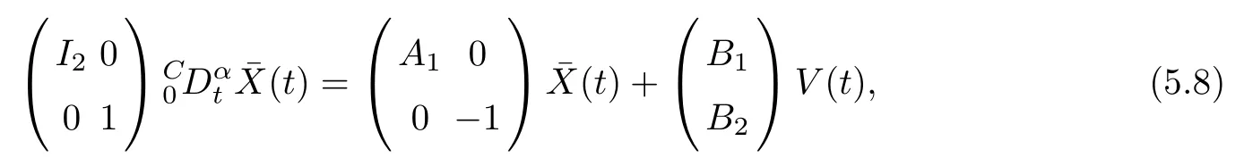
which can be written as

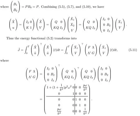
Hence,we conclude that the fractional singular control system(5.1)is changed into another standard fractional control system (5.9), which minimizes the new cost functional (5.11). For the new fractional optimal control problem, define the Hamiltonian function as

The necessary optimality conditions are

Once λ1(t) and λ2(t) are known, we can obtain the optimal control by (5.5) and (5.12) as follows:

The optimal trajectories are

6 Numerical Simulation

In this section, numerical simulation is introduced to verify the theoretical results of the previous sections. We mainly refer to the numerical algorithms in [42]and [43]. Here we do not repeat them. For convenience, we fix the parameter values r = 0.65,d = 200,a1= 0.13,a2=0.2,n1=6,n2=1,q =0.5,m1=1.5,m2=0.45,p=8;c=80. x(0)=1, y(0)=5.

Letting α=0.9, s=0.6, k =5, the solution of linear matrix inequalities (4.5) and (4.6) is

System (4.4) is stable.

For k =1, α=0.9, system (4.4) is also stable, where

For k =1, α=1.4, the solution of (4.7) is

and system (4.4) is stable.

It is worth noting that the scope of k is not easy to obtain, however, by simulation, we know that when α = 0.7, system (4.4) is stable for 0 < k < 20, however, it does not hold for α = 1.2. This means that, for singular fractional system, α > 1 is more complex and hard to stabilize.

From Figure 1 and Figure 2,model system(4.4)can be stabilized around P4(x∗,y∗,E∗)and the singularity induced bifurcation is eliminated. Moreover, when α=1.3, the speed at which the system reaches the equilibrium point is significantly faster than that of α = 0.8. Figure 3 shows the impact of different α on convergence;the greater the α, the faster the convergence.

Figure 1 Dynamic responses of system (4.4) for α=0.8 (a2 =0.6,s=0.4,p=0.8,k =5)

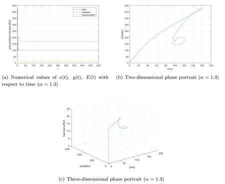
Figure 2 Dynamic responses of system (4.4) for α=1.3 (a2 =0.6,s=0.4,p=0.8,k =5)

Figure 3 Dynamic responses of system (4.4) for different α (a2 =0.6,s=0.4,p=0.8,k =5)

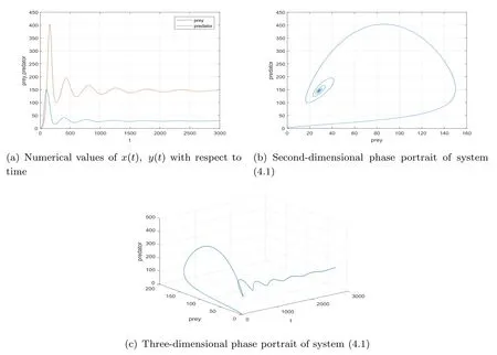
Figure 4 Numerical values of x(t), y(t) for system (4.1) (k =5, s=0.4, α=0.65)

Figure 5 Numerical values of x(t), y(t) for system (4.1) (k =5, s=0.4, α=0.9)

Again, the fractional order index α also influences the the asymptotic stability. Under the given parameter values (here let s=0.4 in order to obtain a more obvious state change),there only exists one equilibrium point of P3, which is P3= (28.7648,148.8238,0). According to Theorem 4.3, we calculate that ∆′= −0.2722< 0, Q1= 0.0330> 0, arctanfor α=1.1,which all satisfy (iii) of Theorem 4.3. Hence, we obtain the locally asymptotic stability of P3. The numerical simulation can be seen in Figure 4, Figure 5 and Figure 6.

In addition,in Figure 7,Figure 8 and Figure 9,simulation results show the periodic solutions of the system for different α,and the period of the solutions increases as α decreases. In practical applications,this tells us that we should choose the right time for harvesting,which is conducive to the sustainable development of ecosystems.

Figure 10 and Figure 11 show the numerical simulations of the optimal control problem for system (5.1). From Figure 10 (a) and Figure 11 (a), we know that system (5.1) is stable after the introduction of feedback control. Figure 10(b)and Figure 11(b)demonstrate the behaviors of the adjoint system, and optimal control u can be seen from Figure 10 (c) and Figure 11 (c).Obviously, the cases in which α =0.8 and α =1.3 are much different, not only from the states x(t),y(t),E(t), but also from the adjoint systems, which also influences the optimal control u.

Figure 8 Numerical values of x(t), y(t) for system (4.1) (s=0.05, α=0.85)

Figure 9 Numerical values of x(t), y(t) for system (4.1) (s=0.05, α=1.1)

Figure 10 Numerical simulations for the optimal control problem of system (5.1) for α=0.8

Figure 11 Numerical simulations for the optimal control problem of system (5.1) for α=1.3

7 Concluding Remarks

In this article, a fractional order singular Leslie-Gower prey-predator model has been established. Dynamical behavior of the system has been extensively investigated, and it has been shown that the singularity induced bifurcation occurs as the economic profit increases through 0, and impulsive behavior emerges which causes a rapid growth of the species population and ecosystem collapse. This unbalanced phenomenon can be eliminated by (optimal)control strategies applied through theory analysis. Finally, the corresponding numerical simulations have been given to verify the feasibility of the results. Moreover, the theoretical and numerical results presented in this article show that the dynamic behavior of the system is not only affected by economic interests, but is also complicated on account of the existence of fractional order derivatives.