Interannual Variability and Scenarios Projection of Sea Ice in Bohai Sea Part I: Variation Characteristics and Interannual Hindcast

JIAO Yan , HUANG Fei , LIU Qingrong, LI Ge, LI Yaru, YU Qingxi,and ZHAO Yiding

1) Key Laboratory of Physical Oceanography, Institute for Advanced Ocean Study, Ocean University of China,Qingdao 266100, China

2) North China Sea Marine Forecast Center, Qingdao 266061, China

3) Laboratory for Ocean and Climate Dynamics, Pilot National Laboratory for Marine Science and Technology(Qingdao), Qingdao 266237, China

4) North China Sea Data & Information Service, Qingdao 266061, China

Abstract The Bohai Sea is one of the southernmost areas for sea ice formation in the northern hemisphere. Sea ice disasters in this body of water severely affect marine activities and the safety of coastal residents. In this study, we analyze the variation characteristics of the sea ice in the Bohai Sea and establish an annual regression model based on predictable mode analysis method. The results show the following: 1) From 1970 to 2018, the average ice grade is (2.6±0.8), with a maximum of 4.5 and a minimum of 1.0.Liaodong Bay (LDB) has the heaviest ice conditions in the Bohai Sea, followed by Bohai Bay (BHB) and Laizhou Bay (LZB). Interannual variation is obvious in all three bays, but the linear decreasing trend is significant only in BHB. 2) Three modes are obtained from empirical orthogonal function analysis, namely, single polarity mode with the same sign of anomaly in all of the three bays and strong interannual variability (82.0%), the north–south dipole mode with BHB and LZB showing an opposite sign of anomalies to that in LDB and strong decadal variations (14.5%), and a linear trend mode (3.5%). Critical factors are analyzed and regression equations are established for all the principal components, and then an annual hindcast model is established by synthesizing the results of the three modes. This model provides an annual spatial prediction of the sea ice in the Bohai Sea for the first time,and meets the demand of operational sea ice forecasting.

Key words sea ice; Bohai Sea; variation characteristics; interannual hindcast; predictable mode analysis

1 Introduction

The Bohai Sea is one of the southernmost latitudinal areas for sea ice formation in the northern hemisphere.Severe sea ice conditions in this body of water directly affect marine transportation, fishery, oil and gas exploitation, marine ecology, and the safety of coastal residents(Zhang, 1982; Zhang and Gao, 2015). As shown in Fig.1,the sea ice is mainly distributed in Liaodong Bay (LDB),Bohai Bay (BHB), and Laizhou Bay (LZB) of the Bohai Sea, and the ice period is approximately four months per year (Deng, 1985; Bai and Liu, 1999). As climatic conditions change from year to year, strong interannual variability of sea ice occurs in the Bohai Sea. Based on the extent and thickness of the ice, the ice condition is divided into five grades (Criteria for Forecasting Grades of Sea Ice in China, 1973): grades 1–5 represent very mild, mild, normal, heavy, and very heavy ice conditions. Sea ice grade with an accuracy of 0.5 is typically used in practical forecasting. According to historical records, serious sea ice disasters occurred in the Bohai Sea in 1969 (1968/1969 winter, the same below), 1977, 2001, and 2010. At the worst, the Bohai Sea was almost icebound, which had a serious impact on the lives and productivity of coastal and island residents, and also caused huge economic losses(Sun et al., 2010). Therefore, studying sea ice variations and its driving factors in the Bohai Sea is important, as well as making accurate predictions to reduce the detrimental socioeconomic effects of sea ice disasters.

At present, the interannual prediction of the sea ice in the Bohai Sea mainly depends on statistical prediction.By analyzing the relationship between tropical Pacific sea surface temperature (SST) and the sea ice grades in the Bohai Sea, Xie et al. (1991) found out that when El Niño events occur, warm weather usually occurs in north and northeast China in the following winter, thereby causing a mild ice year. Xie et al. (1991) selected two key areas from the tropical Pacific Ocean and estimated a multiple regression equation to predict sea ice grade in winter,thereby achieving a quantitative forecast of sea ice grade for the first time. Li et al. (2009) found that the sea ice grade is significantly correlated with the Pacific subtropical high (PSH), and built a linear equation using PSH intensity index in August to predict the sea ice grade.Based on the findings of Li et al. (2009), Tang et al.(2015) proposed that the Siberian high is another important factor that affects the interannual variation of sea ice in the Bohai Sea, and established a binary regression equation with the SH and PSH intensity indexes. Furthermore, Zheng et al. (2015) and Jiao et al. (2017) used stepwise regression and teleconnection analysis, respectively, to select factors and established forecast equations to predict the sea ice grade in the Bohai Sea. It can be seen that, almost all interannual predictions focus on the overall ice condition or ice grade. However, the ice conditions in the three frozen sea areas (i.e., LDB, BHB, and LZB) are obviously different, and the overall prediction at present cannot reflect the ice characteristics of each bay.Thus, current predictions are unable to meet the requirements for the prevention and mitigation of sea ice disasters.

Predictable mode analysis (PMA) was proposed by Wang et al. (2007). The PMA method assumes that if the first several modes of an interannual variation signal obtained by empirical orthogonal function (EOF) analysis can reflect the main changes of the signal, and can be predicted by a set of physics-based empirical (P-E) models, then they are called predictable modes. The PMA method can predict the interannual variation of spatial distribution of the predictand. Xing et al. (2016) used the PMA method to predict the precipitation anomaly in the East Asian summer monsoon area four months in advance,and the prediction skill is twice higher than that of the dynamical model hindcast. In this study, the PMA method is used to predict the spatial distribution of interannual variation of the sea ice in the Bohai Sea.

The paper is organized as follows: Section 2 introduces the data and research methods. Section 3 analyzes the interannual variation characteristics of sea ice in the Bohai Sea. Section 4 establishes the regression model of sea ice based on PMA method. Section 5 summarizes the major results and discusses the following work.

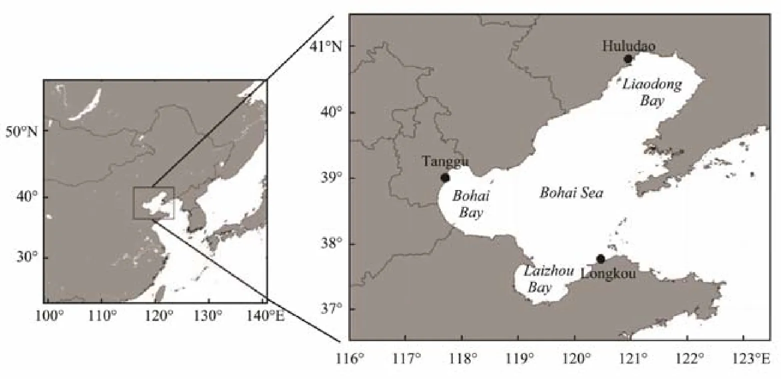
Fig.1 Map of Bohai Sea and locations of representative ocean stations.

2 Data and Methods

2.1 Data

A historical sea ice dataset is used to analyze the interannual and long-term variation characteristics of sea ice in the Bohai Sea. The dataset includes sea ice grades and the maximum distance from the shore to the edge of the sea ice along the baseline (SIE) in LDB, BHB and LZB from 1970 to 2018. SIE is the prediction variable of the sea ice in China, and the measurement baselines for LDB, BHB,and LZB are defined as (121˚52΄E, 40˚52΄N–120˚00΄E,39˚00΄N), (117˚33΄E, 38˚42΄N–120˚00΄E, 38˚25΄N), and(119˚18΄E, 37˚07΄N–119˚50΄E, 38˚00΄N), respectively. The dataset is provided by the North China Sea Marine Forecast Center (NCSMF).

Ocean station observations are used to study the influence of local marine and meteorological factors on the sea ice. Monthly mean air temperature (AT) and SST observation data of three ocean stations along the coast of the Bohai Sea, namely, Huludao (HLD), Tanggu (TGU), and Longkou (LKO) from 1969 to 2018 are used, which are also provided by the NCSMF.

Monthly reanalysis data from NCEP/NCAR and Had-ISST from the UK Met office are used to establish the regression model and explain the physical mechanism.The data set covers the period from 1969 to 2018.

2.2 Methods

The PMA method is a complete prediction system that includes statistical analysis, physical mechanism, and hindcasting test. In this study, EOF analysis of SIE in the three frozen areas in the Bohai Sea from 1970 to 2018 is first performed to obtain the spatial patterns and principal components (PCs) of the main modes. Then, the P-E models of each mode are established and tested. Finally, the predictions of each mode are added by variance weight to obtain the final results of SIE in the three areas of the Bohai Sea.

We also apply correlation analysis, stepwise regression analysis, and other methods to select factors, explain physical mechanisms, and establish the P-E models. Furthermore, cross-validation method is used to test the generality and stability of the P-E models.

3 Variation Characteristics of Sea Ice

In Section 1, we introduced the concept of sea ice grades to describe the overall ice severity in the Bohai Sea. Fig.2 shows the interannual variations of ice grades from 1970 to 2018. During that period, the average ice grade was(2.6±0.8) with a maximum of 4.5 in 1977 and a minimum of 1.0 in 1973, 1995, 2002 and 2015. In terms of occurrence times, grade 3.0 occurs most often (17 times), followed by grades 2.0 and 2.5 (9 and 8 times, respectively).

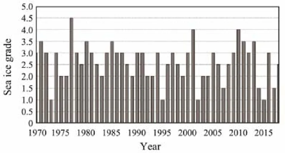
Fig.2 Interannual variation of sea ice grades from 1970 to 2018.

As the ice grade is an overall description of the ice condition, it cannot reflect the difference of ice conditions in each frozen sea area. Therefore, we select the maximum SIE in each area to represent the sea ice intensity in each bay. Through this approach, we can further analyze the variation characteristics of the sea ice in the Bohai Sea.

Figs.3a–c show the variations of SIE in LDB, BHB, and LZB. Among the three bays in the Bohai Sea, LDB is characterized by the heaviest sea ice. The mean value of SIE from 1970 to 2018 is (70.5±18.2) nautical miles (n mile). The maximum value was 118 n mile, which occurred in 1977, while the minimum value was only 38 n mile, which occurred in 1973 and 1995. Taking 1 standard deviation greater/less than the mean value as the criterion for judging a heavy/mild ice year, we found that 6 heavy ice years and 9 mild ice years occurred in LDB during the study period.

Sea ice in BHB is milder than that in LDB. The mean value of SIE is (18.7±11.7) n mile. The maximum value was 60 n mile, which also occurred in 1977, while the minimum value was 0 n mile, which meant that no sea ice formed in 1973, 1995, and 2015. A total of 9 heavy ice years and 6 mild ice years occurred from 1970 to 2018.

LZB is the sea area with the mildest ice condition in the Bohai Sea. The mean value of SIE is (16.1±12.8) n mile,with a maximum of 46 n mile in 2010, and a minimum of 0 n mile in 1973, 1995, 2015, and 2017. From 1970 to 2018,a total of 8 heavy ice years and 5 mild ice years were observed. Notably, the ice condition in LZB is weaker than that in BHB, but the standard deviation of SIE is larger.The reason is that, due to the influence of geographical location, when the sea ice in BHB melts in late winter in some years, the floating ice is driven by the sea surface wind toward LZB. As a result, the sea ice used to measure SIE in LZB comes from BHB because of wind instead of originating within LZB, thereby leading to a larger measured value of SIE and its standard deviation in LZB.

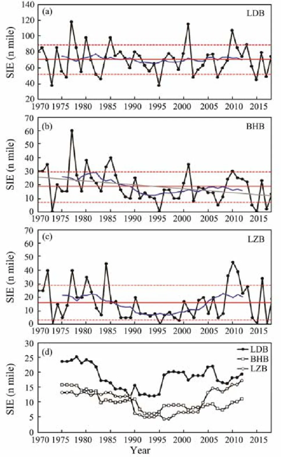
Fig.3 Interannual and decadal variations of SIE (a–c) and 11-year sliding standard deviations (d) in LDB, BHB,and LZB.

Table 1 shows the correlation coefficients of SIE between the three frozen bays. The best correlation is between LDB and BHB with a correlation coefficient of 0.80,followed by BHB and LZB with 0.77, and then LDB and LZB with 0.60. The correlation coefficient also reflects the location and geographical latitude of each bay.

From a long-term perspective, only BHB has a significant downward trend with a decline rate of 2.9 n mile/10 year (P < 0.01), whereas the trend in LDB and LZB is not significant. From a decadal perspective, all bays show an inverted Ω distribution, with two peaks around 1982 and 2008, and one valley around 1993.

Fig.3d shows a time series of 11-year sliding standard deviations that reflect decadal variations of ice oscillation intensity. The interdecadal variation trend of ice oscillation intensity is similar to that of ice intensity. From the 1970s to the 1990s, the amplitude of ice oscillation decreased, whereas from the 1990s to the present, the intensity of ice oscillation increased. This is an important variable that needs further attention because during periods of strong ice oscillation, changes in ice conditions have a high likelihood of causing unexpected sea ice disasters and economic losses.

Table 1 Correlation coefficients of SIE among three frozen bays

4 Interannual Hindcast Model of Sea Ice

4.1 EOF Analysis

The interannual variation of SIE in the Bohai Sea is decomposed by EOF analysis to obtain the spatial patterns and PCs. As shown in Fig.4, the first mode, which is called single polarity mode with the same sign of anomaly in all three bays, represents the consistent changing of the sea ice in the three bays dominated by LDB, thereby explaining 82.0% of the interannual variance. The second mode, which is called north–south dipole mode, is where BHB and LZB have the opposite sign of anomalies to that in LDB; this mode explains 14.5% of the total variance.The third mode is dominated by BHB. As shown in the following, this mode can be called linear trend mode,which explains 3.5% of the total variance.

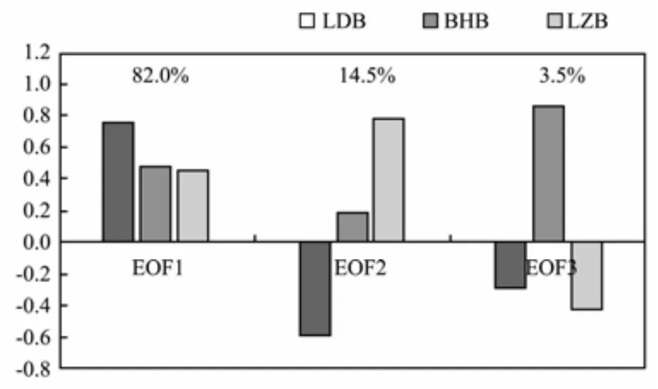
Fig.4 Spatial patterns and variance contribution of EOF modes.

4.2 Single Polarity Mode

The first mode of EOF analysis represents the consistent change of the sea ice in the Bohai Sea. From a global point of view, the area of the Bohai Sea is very small, with a 4˚ span in latitude and longitude. Therefore, the single polarity mode accounts for most of the variance contributions (82%).

In this section, cross-lagged correlation analysis between PC1 and surface temperature is first used to select the key areas and define the indices. Then, the indices are screened by stepwise regression and the physical mechanism is explained. Finally, we establish the P-E model and use the cross-validation method to test the generality and stability of the model.

The cross-lagged analysis shows that the best correlation appears in November, that is, one month before the sea ice period. Fig.5b shows a correlation map between PC1 and AT in November. In the AT correlation map, the two key areas are located in west of the Ural Mountains(35˚–50˚N, 20˚–50˚E) and eastern Eurasia (20˚–45˚N,100˚–125˚E). The mean ATs of the two areas are defined as the prediction indices, which are called AT_WU and AT_EA, respectively. Considering that both of the key areas are located in Eurasia, the difference between AT_WU and AT_EA is also taken as one of the prediction indices, called AT_WU-EA. Fig.5c presents a correlation map between PC1 and SST. The three key areas are the following: tropical Central Pacific (10˚S–15˚N, 160˚E–170˚ W), southern Gulf of Alaska (40˚–60˚N, 150˚–125˚W),and southwest to Australia (30˚–45˚S, 110˚–130˚E). The mean SSTs of these key areas are defined as another three prediction indices, which are called SST_CP, SST_AK,and SST_AUS.

As we have defined as many predictors as possible without considering the correlation between them, we adapt the stepwise regression method to select the impact factors. The factors obtained from the stepwise regression are AT_WU-EA, SST_CP, and SST_AUS. The physical mechanism of each index is explained in the following.

Fig.6 shows the regressed 500 hPa geopotential height by AT_WU-EA index. As the figure shows, one month before the sea ice period, the regression coefficient over Eurasia exhibits a “-+-” distribution, that is, a negative anomaly over Scandinavia, a positive anomaly over the Ural mountains, and a negative anomaly over eastern Eurasia. The structure is similar to the positive phase of the Eurasian teleconnection (EU). The influence of this distribution on the sea ice is that, when EU is in a positive phase, the Ural blocking high strengthens and the geoposition height over eastern Inner Mongolia decreases.This condition indicates a meridional circulation over Eurasia, and the East Asia trough deepens and moves westward. This situation is favorable for the cold air from Siberia to move southeastward along the steering flow,thereby resulting in the negative AT anomaly in Northeast China. The conclusion is consistent with the findings of Huang and Gao (2012), Liu and Chen (2012), and Zuo and Xiao (2013).

When the positive phase of EU is maintained in the upper air, the AT anomaly on the west side of the Ural mountains is positive due to the southerly wind anomaly,while the AT anomaly in East Asia is negative due to the northerly wind anomaly. Therefore, the AT_WU-EA index represents the influence of mid-high latitude circulation on the sea ice in the Bohai Sea.

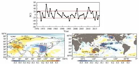
Fig.5 PC1 and its correlation coefficient map with surface temperature in November: (a) PC1, (b) correlation coefficient with 2 m AT, and (c) correlation coefficient with SST. The dotted red line represents ±1σ. The black dot is the area where P < 0.05. The red boxes indicate the areas where predictors are defined.

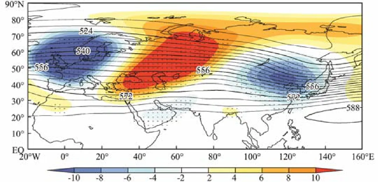
Fig.6 Geopotential height of 500 hPa (contour) and regressed geopotential height by AT_WU-EA index (shaded). The black dot is the area where P < 0.05.

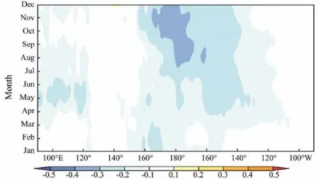
Fig.7 Relation between PC1 and evolution of SST in tropical Pacific (10˚S–15˚N) from January to December of the year before sea ice period.

The second key area, which is located in the tropical Central Pacific, represents the occurrence of El Niño/La Niña Modoki. Fig.7 shows the relation between PC1 and the evolution of SST in the tropical Pacific (10˚S–15˚N)from January to December of the year before the sea ice period. The signal of SST anomaly occurs in July and reaches its peak in October and November. In other words,when the La Niña/El Niño Modoki event occurs in the autumn, the sea ice in the Bohai Sea is heavy/mild in the following winter. Some studies have shown that El Niño/La Niña has a certain impact on winter climate in China and ice conditions in the Bohai Sea. Shen and Wang (2018)pointed out that ENSO Modoki index is positively correlated with the temperature in Northeast China. Geng and Wang (2001) found that during La Niña years, the West PSH weakens and the polar vortex divides, thereby resulting in an enhanced meridional circulation over East Asia and increased ice intensity in the Bohai Sea.

The area of SST_AUS is located southwest of Australia in the southern hemisphere. The regressed 700 hPa geopotential height by SST_AUS shows a typical southern hemisphere annular mode (figure not shown). Huang et al.(2011) pointed out that the annular modes of the northern and southern hemispheres are in the same phase in the interannual variability, which may be connected through the ‘atmospheric bridge’ of the transhemispheric tele- correlation wave train. Wu et al. (2009) proposed that the southern hemisphere annular mode affects China winter monsoon through Hadley circulation. The physical mechanism of SST_AUS on the sea ice in the Bohai Sea needs further research. However, as the third predictor, this key area represents the influence of the interaction between the northern and southern hemispheres on the sea ice in the Bohai Sea.

Based on the three indices, the following P-E model for PC1 is established:

The observed (black line) and regressed (blue line) PC1 are shown in Fig.8, and the correlation coefficient is 0.68,which is significant at the 99% level. To prove the generality and stability of the model, the cross-validation method is used to make a retrospective forecast for PC1. We leave out three years of data progressively, and then train the model using the data of the remaining years and finally apply the model to forecast for the three years. The predicted PC1 using the cross-validation method is shown by the red line in Fig.8, and its correlation coefficient with the observation is 0.63, which is also significant at the 99%level. Therefore, EOF1 is proven to be a predictable mode.

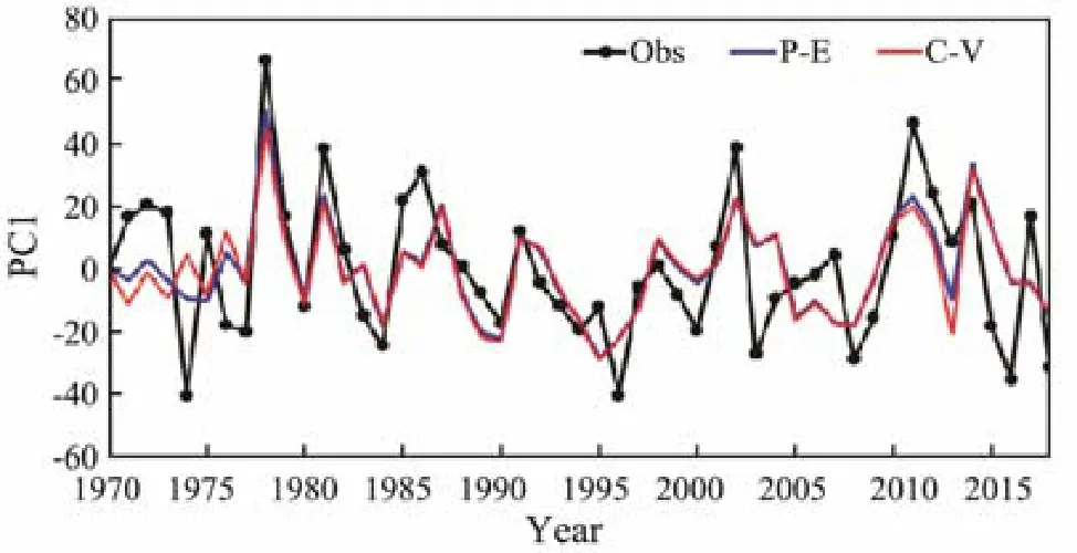
Fig.8 Comparison of PC1 in observation (black line), regression (blue line), and cross-validation prediction (red line).

4.3 North–South Dipole Mode

The north–south dipole mode is the second mode of EOF analysis. No significant correlation exists between PC2 and the large-scale circulation (the figure abbreviated),indicating that the Bohai Sea is a small area where the difference between the north and south of the sea ice is mainly determined by the local marine and meteorological factors rather than the large-scale circulation factors.Thus, we study the relationship between local temperature and PC2 in the Bohai Sea before the sea ice period.

Three ocean stations, namely, HLD, TGU, and LKO,with long-time continuous observation data, are selected as the representative stations of LDB, BHB, and LZB,respectively. According to the locations of the ocean stations, we defined six indices of AT and SST, namely,HLD, TGU, LKO, HLD-TGU, HLD-LKO, and HLD-1/2(TGU+LKO).

Fig.9b shows the monthly variation of the correlation coefficient between PC2 and the SST indices (no SST data were available from January to March due to icing).We can observe that sea ice severity in winter is well correlated with SST in spring and early summer. From April to July, SST in TGU is negatively correlated with PC2, and the correlation is the strongest in May. From April to July,the difference of SST between HLD and TGU is positively correlated with PC2, with the strongest correlation in June. From June to July, SST of HLD-1/2(TGU+ LKO)is positively correlated with PC2 and also shows the strongest correlation in June. This result indicates that the local signal of the SST anomaly in spring and early summer could be stored and is reflected in the ice condition in the following winter. Therefore, three indices are selected as possible factors, namely, TGU_SST_MAY, HLD-TGU_SST_JUN, and HLD-1/2(TGU+LKO)_SST_ JUN.

Fig.9c shows the monthly variation of the correlation coefficient between the PC2 and AT indices. As the figure indicates, the correlation between AT and PC2 is obviously lower than that of SST. Only the AT of HLD-LKO in September is significantly related to sea ice in winter,thereby indicating that compared with sea water, the atmosphere has poor ability to store heat. HLD-LKO_AT_SEP is selected as the fourth index.

As the indices are not independent, a stepwise regression method is used again to select the prediction factors,and the P-E model is established as follows:

The observed (black line) and regressed (blue line) PC2 are shown in Fig.10, and the correlation coefficient is 0.53, which is significant at the 99% level. The predicted PC2 using the cross-validation method is indicated by the red line and its correlation coefficient with the observation is 0.49, which is also significant at the 99% level.Therefore, EOF2 is proven to be a predictable mode.

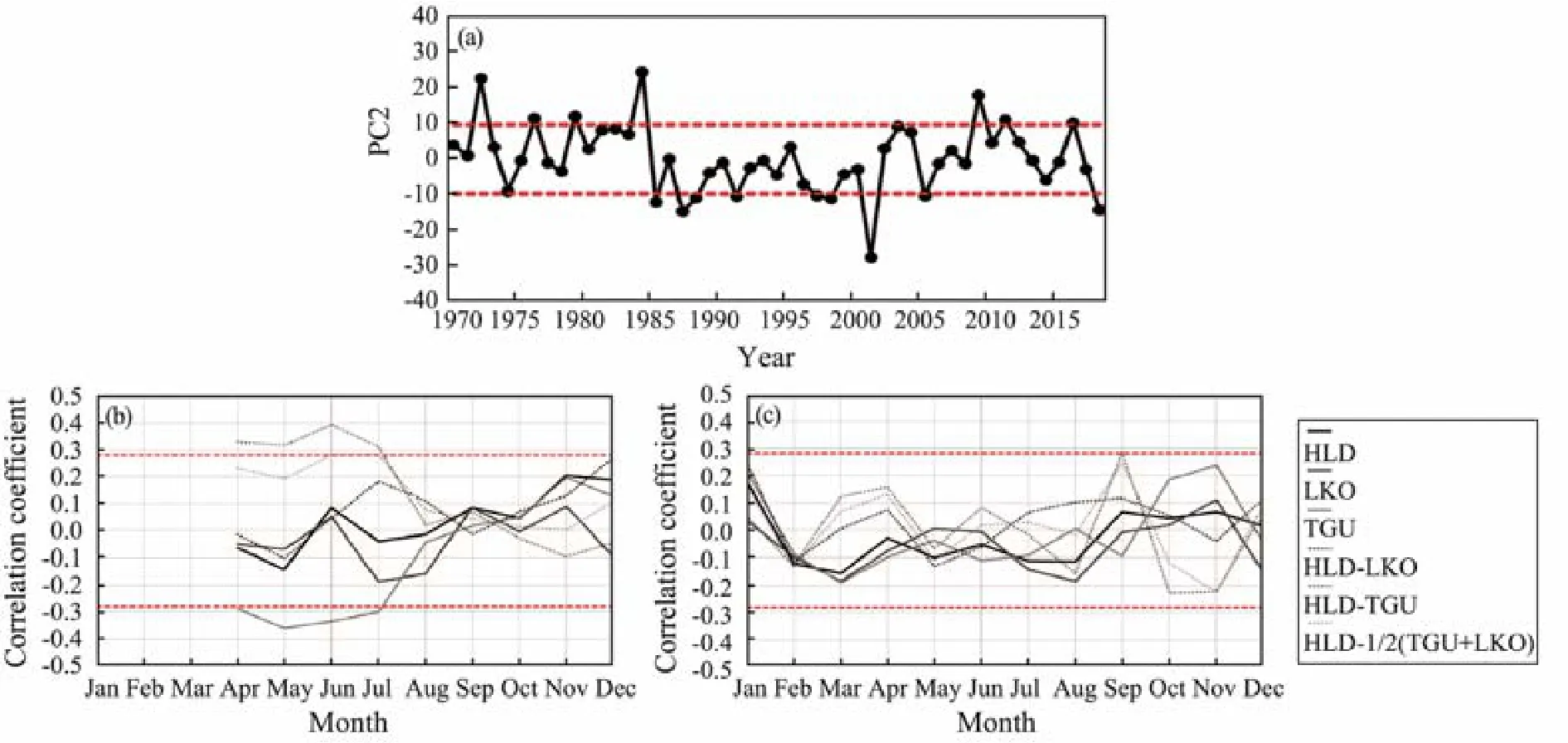
Fig.9 PC2 and its monthly variation of correlation coefficient with local surface temperature: (a) PC2; the dotted red line represents ±1σ. (b–c) Correlation coefficient with SST and AT; the dotted red line represents the significance at 95% level.

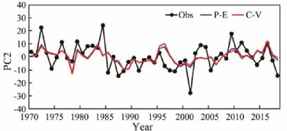
Fig.10 Comparison of PC2 in observation (black line),regression (blue line), and cross-validation prediction(red line).

4.4 Linear Trend Mode

Fig.11 shows the variation of PC3 and its linear trend.Combined with the spatial pattern of EOF3, this mode represents a long-term decline trend dominated by the sea ice in BHB, which is consistent with the results in Section 3.

As the linear decline trend of PC3 is significant at the 99% level, this mode is also a predictable mode. We use the linear fitting equation of PC3 directly as the regression equation of PC3, and the correlation coefficient is 0.57.

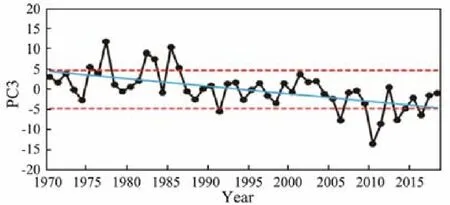
Fig.11 PC3 and its linear trend (blue line). The dotted red line represents ±1σ.

4.5 Reconstruction Result of Each Bay

Based on the regressed PCs, the sea ice in the Bohai Sea can be calculated by using the sum of the three spatial patterns multiplied by the corresponding regressed PCs.As shown in Fig.12, the correlation coefficients between the observation and reconstruction are 0.67, 0.74, and 0.59 in LDB, BHB, and LZB, respectively, which can meet the requirements of operational sea ice forecasting.

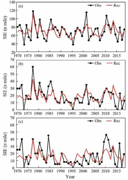
Fig.12 Comparison of SIE in (a) LDB, (b) BHB, and (c)LZB in observation (black line) and reconstruction (red line).

5 Discussion and Conclusions

In this study, we first analyzed the characteristics of sea ice interannual variability in the Bohai Sea, including sea ice grade and SIE in the three frozen bays. Then, using the PMA method, we constructed a hindcast model of sea ice in each of the bays. In all the three areas, the modelbased SIE reconstruction showed a statistically significant correlation with historical observations. This model may be used for operational sea ice forecasting.

From 1970 to 2018, the average ice grade was (2.6 ±0.8), with a maximum of 4.5 and a minimum of 1.0, and grade 3.0 occurred most often.

The sea area with the heaviest ice condition in the Bohai Sea was LDB, where the mean value of SIE was (70.5 ±18.2) n mile, followed by BHB with (18.7 ± 11.7) n mile and LZB with (16.1 ± 12.8) n mile. A significant interannual variation of sea ice occurred in the three bays, but the linear decreasing trend was significant only in BHB.

Based on the EOF analysis of historical data from 1970 to 2018, three modes of variability were obtained, namely,1) the single polarity mode with the same sign of anomaly in the three bays and with variability on interannual timescales (which explained 82.0% of the interannual variance); 2) the north–south dipole mode where the BHB and LZB had the opposite sign of anomalies to that in LDB and showed a significant variation on decadal timescales (which explained 14.5% of the interannual variance); and 3) the linear trend mode (which explained 3.5% of the total variance). Correlation analysis between PC1 and surface temperature was used to define key areas and indices, and a stepwise regression analysis was conducted to select the prediction factors. The selected factors were AT_WU-EA, SST_CP, and SST_AUS, which represented the effects of the EU teleconnection in the middle and high latitudes in the northern hemisphere, the El Niño/La Niña Modoki in the tropical Pacific Ocean,and the interaction between the northern and southern hemispheres on the sea ice in the Bohai Sea, respectively.The correlation between the reconstruction based on the P-E model and PC1 from observations was significant (R= 0.68, P < 0.01). The second mode of EOF represented the north–south dipole changes in the sea ice. As the Bohai Sea occupies a small area, we mainly considered the effect of local marine and meteorological factors on the sea ice in the Bohai Sea. Through lagged cross correlation analysis and stepwise regression, the predictors of PC2 were obtained as HLD-TGU_SST_JUN and HLDLKO_AT_SEP. The correlation coefficient between the reconstructed value of P-E model and the observation of PC2 was 0.53 (P < 0.01). The third mode of EOF was the linear trend mode of the sea ice in the Bohai Sea, and the correlation coefficient between the P-E reconstruction and PC3 was 0.57 (P < 0.01), which was again statistically significant.

The SIE in each bay can be calculated by using the sum of the three spatial patterns multiplied by the corresponding reconstructed PCs. The correlation coefficients between the construction and observations were 0.67, 0.74,and 0.59 in LDB, BHB, and LZB, respectively, which were statistically significant and could potentially meet the demands of operational sea ice forecasting.

However, the skill of sea ice reconstruction in LZB was lower than that in the other two bays. The reason was that,during melting period in some years, sea ice in BHB would drift to LZB under westerly winds such that SIE measured in LZB would include not only the sea ice formed locally in the bay but also those from other areas. Therefore, to improve regression model skills, we have to examine the interactions of sea ice from different areas in the following work.

In terms of finding the most critical predictors, EOF1 reflects the influence of large-scale atmospheric circulation on the sea ice in the Bohai Sea. However, the physical mechanism underlying the interaction between the northern and southern hemispheres needs further investigation. The second mode mainly reflects the influence of local marine and meteorological forcing. However, we have to further study the seasonal variations in correlations between the SST and PC2, namely, high in spring and early summer but low in autumn.

Acknowledgements

The study is supported by the National Natural Science Foundation of China (Nos. U1706216 and 41575067) and the National Key Research and Development Program(Nos. 2015CB953904, 2016YFC1402000, and 2016YFC 1401500).