A statistical inference for generalized Rayleigh model under Type-II progressive censoring with binomial removals

REN Junru and GUI Wenhao

Department of Mathematics,Beijing Jiaotong University,Beijing 100044,China

Abstract: This paper considers the parameters and reliability characteristics estimation problem of the generalized Rayleigh distribution under progressively Type-II censoring with random removals, that is, the number of units removed at each failure time follows the binomial distribution. The maximum likelihood estimation and the Bayesian estimation are derived. In the meanwhile,through a great quantity of Monte Carlo simulation experiments we have studied different hyperparameters as well as symmetric and asymmetric loss functions in the Bayesian estimation procedure.A real industrial case is presented to justify and illustrate the proposed methods.We also investigate the expected experimentation time and discuss the influence of the parameters on the termination point to complete the censoring test.

Keywords: Type-II progressive censoring with random removals,generalized Rayleigh distribution, reliability characteristic, maximum likelihood estimation, Markov chain Monte Carlo method,expected experimentation time.

1.Introduction

At present, the lifetime of a product,or the quality,is the determined factor for an enterprise to obtain great market share. Improving the quality inspection not only has important benefits for enterprise development,but also has a profound effect on our society.Reliability is an important index to judge product quality. In recent years, the interaction between reliability and statistical data has become a popular trend,extensively studied by many statisticians.It is necessary for us to conduct the statistical inference of the lifetime distribution parameters and reliability characteristics.

In life testing experiments,it is commonly assumed that we can obtain and observe a complete sample, based on which a series of statistical inferences are given. In the real life,however,due to a variety of reasons,such as the time constraint, lack of funds, the insufficiency of material sources or the difficulty of testing and so on,censored samples may arise.

Suppose thatr1,r2,...,rmunits are removed at each failure time respectively,wherer1,r2,...,rmare specific values which are known in advance. The process above is the Type-II progressive censoring scheme.It is obvious that, the complete sample (r1=r2=···=rm= 0)and the conventional Type-II right censored sample(r1=r2=···=rm-1=0,rm=n-m)are the special cases of the Type-II progressive censoring scheme.

This type of sampling method has received great attention, especially in the analysis of lifetime data. Ali et al. [1] discussed the maximum likelihood estimation and Bayesian estimation of the parameter of Rayleigh distribution under progressively Type-II censoring.Chien et al.[2]obtained the maximum likelihood estimation of the Log-Gamma distribution using the expectation-maximization(EM) algorithm. Singh et al. [3] not only considered the classical and Bayesian methods of parameter estimation of the inverse exponential distribution,but also studied the estimation of the reliability function and the efficiency function.

However,notice thatr1,r2,...,rmare fixed and given in advance, the Type-II progressive censoring scheme does not have the flexibility of allowing random removals at each failure time. The numbers of units removed,r1,r2,...,rm, are specific values that are all pre-fixed.However,products may be removed unexpectedly and accidentally in practice.It motivates and leads us into the area of progressively Type-II censoring with random removals.

For further related study about Type-II progressive censoring with the binomial removal scheme, one may refer to the following literature.For example,Dey et al.[4]carried out parameter estimation of the weighted exponential distribution under Type-II progressive censoring with binomial removals, Yan et al. [5] discussed the maximum likelihood estimation and confidence interval of the parameter of the generalized exponential distribution under the censored scheme. Moreover, Dey et al. [6,7] studied statistical inference of the Rayleigh distribution and generalized inverse exponential distribution respectively,including maximum likelihood estimation and Bayesian estimation. Singh et al. [8,9] mainly studied the Bayesian estimation of the Poisson-exponential model and the Rayleigh distribution and its application in the real case.In addition,the studies for the Weibull distribution,exponential distribution,Pareto distribution and Burr type XII can be found in[10–14]respectively.

The two-parameter generalized Rayleigh(GR)distribution introduced in [15] is a special case of the generalized Weibull distribution. Its probability density function(PDF) and hazard function take on different shapes with the change of two parameters,and it can fit various skewed data very well.Moreover,the GR distribution has wide applications in many fields,for instance,the software industry[16],bearings and other industrial devices[17],vacuum electronic components[18]and so on.

Thus, we focus on the statistical inference for the GR distribution under Type-II progressive censoring with binomial removals.The rest of this paper is organized as follows. The concept of Type-II progressive censoring with binomial removals and some properties of the GR distribution are introduced in Section 2.In Section 3,we obtain the likelihood function of the GR distribution under progressively Type-II censoring with binomial removals,then Sections 3.1,3.2 and 4 introduce maximum likelihood estimation and Bayesian estimation respectively. Section 5 considers Monte Carlo simulation,and in Section 6 we analyze a real industrial dataset which follows the GR distribution to illustrate the proposed model.Finally,Section 7 discusses the expected experimentation time,and the final conclusions are drawn in Section 8.

2.Basic knowledge

2.1 Progressively Type-II censoring with binomial removals

First, suppose that the experimenter placesnunits on a life-testing experiment at time zero and onlym(m < n)failures are to be recorded and observed.At the time of the first failure,R1of the survivingn-1 units are randomly removed, and the failure timeX1:m:ncan be recorded.Similarly, when the second failure is observed,R2of the restn-R1-2 units are randomly removed and we can record the dataX2:m:n, as so on, at the time of themth failure, remove all the remaining live units. Suppose thatR1,R2,...,Rmare random variables following the binomial distribution with a probabilityp(0< p <1). The progressively Type-II censoring with the binomial removal scheme can be summarized in Table 1.

Table 1 Type-II progressive censoring with binomial removals

2.2 GR distribution

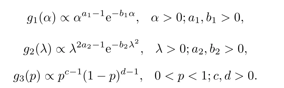
The PDF and cumulative density function(CDF)of the GR distribution are given as follows.

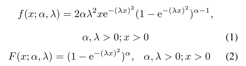
whereαandλare the shape and scale parameters,respectively.The GR distribution is denoted byGR(α,λ).

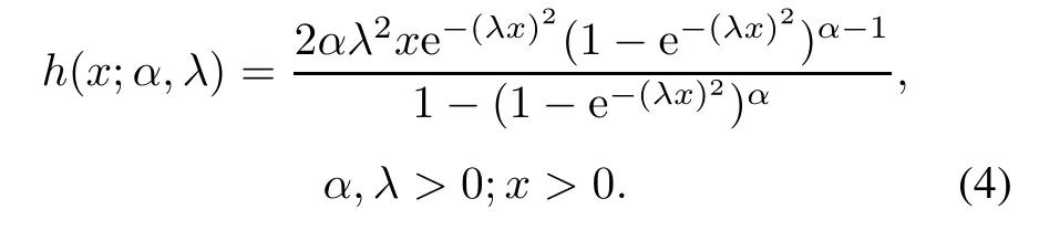
Its survival function is and the hazard function is

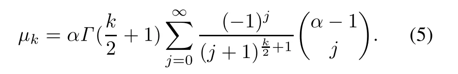
If the random variableXfollows the GR distribution withλ= 1,that is,X ～GR(α,1), then thekth moment[19]ofXis

Raqab et al. [19] pointed out that forα≤ 1/2,the PDF of the GR distribution is a decreasing function, but a right skewed unimodal function forα ＞1/2. In addition, the shape of the hazard function also depends on the parameterα. Forα≤ 1/2, the hazard function presents a bathtub shape, and forα ＞1/2, it is an increasing function. The two-parameter GR distribution has a variety of properties similar to the Gamma distribution and the Weibull distribution. Therefore, it is very suitable for lifetime data fitting. Meanwhile, what is different from other lifetime distributions is that its hazard function is not homogenized,which enhances its applicability greatly.Different forms of the PDF and the hazard function ofGR(α,λ) are presented in Fig.1(a)and Fig.1(b)respectively.

Fig.1 GR distribution

From Fig. 1(b), we can see that forα≤1/2 the hazard function decreases from∞to a positive constant,and then gradually increases to∞, but it will increase from 0 to∞forα ＞1/2.Raqab et al.[19]mentioned,when the shape parameters of the Gamma and Weibull distributions are greater than 1, the hazard functions of them are both increasing functions, and it increases from 0 to 1 for the Gamma,while the Weibull hazard function increases from 0 to∞.In this regard,the properties ofGR(α,λ)are more similar to the Weibull distribution.If a lifetime dataset can be fitted by the Weibull,then GR can also be applied.Forα≤1/2, the hazard function presents the bathtub shape curve,which is common for industrial products.

Through the analysis above, we can see that the GR distribution has various properties and it has already been proved thatGR(α,λ) can be efficient to fit both ordinary and strength lifetime data[20].

Besides,the expected lifetime value E(x)versus parametersαandλcurves are plotted in Fig.2.We can observe that whenλis fixed,E(x)increases asαincreases,but the growth rate decreases gradually.Whenαis fixed, the expected lifetime value E(x)decreases from∞to 0 with the increase ofλ.

Fig.2 Mean value of GR distribution

3.MLE

Assume thatx= (x1:m:n,x2:m:n,...,xm:m:n) is a Type-II progressive censoring sample following the GR distribution,with a binomial removal planR1=r1,R2=r2,...,Rm=rm. The censored sample can be simply written asx=(x1,x2,...,xm),then the conditional likelihood function can be expressed as

whereA=n(n-r1-1)(n-r1-r2-2)···(n-r1-r2-···-rm-1-m+1).

As described earlier, the number of units removed at each failure time is random and independent from each other,and follows the binomial distribution with a probabilityp,so

and fori=2,3,...,m-1,

According to the probability multiplication formula,we have

Substituting(7)and(8)into(9),we obtain

Assuming further thatXiandRiare independent for alli,therefore,the joint likelihood function ofXandRis

where

Note thatCbehaves as a constant for the given data,not depending on the parameters,andL1(α,λ)is a function ofαandλonly,whileL2(p)only involvesp.

3.1 Point estimation

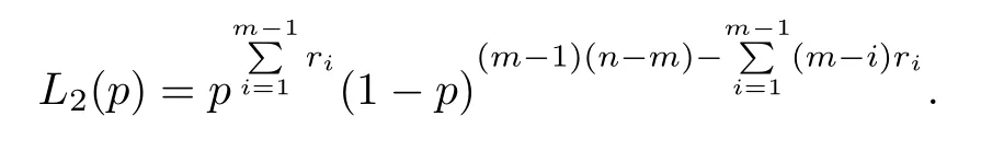
From(11),we know that the maximum likelihood estimators (MLEs) ofαandλcan be obtained by maximizingL1(α,λ),and similarly we can maximizeL2(p)to get the MLE ofp.

The log-likelihood function ofL1is given by

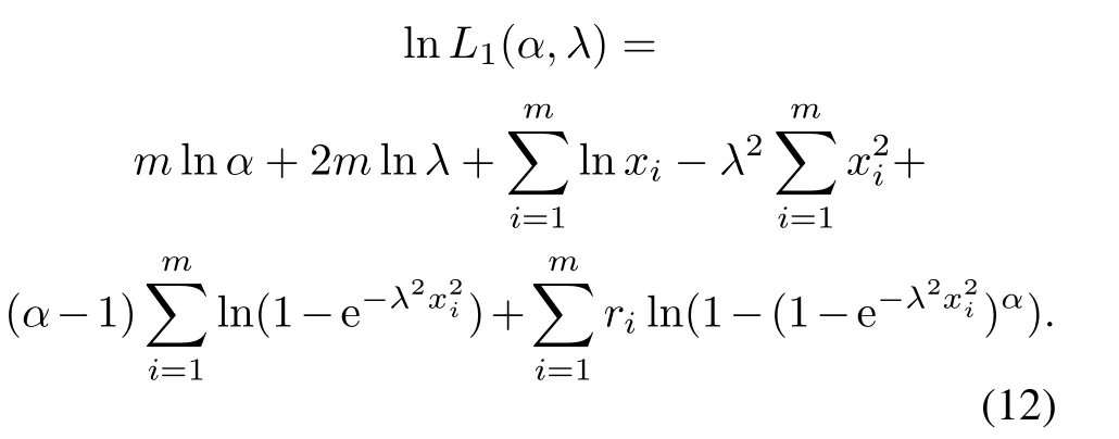
Differentiating(12)with respect toαandλ,we have

where

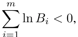
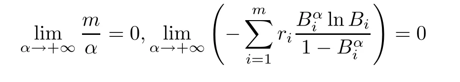
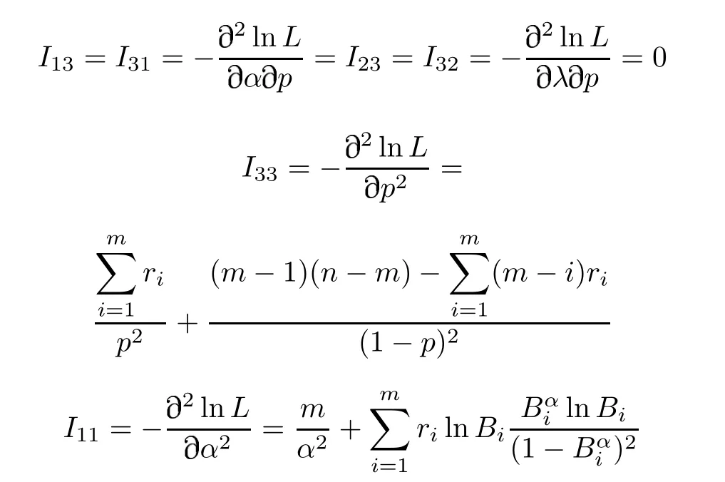
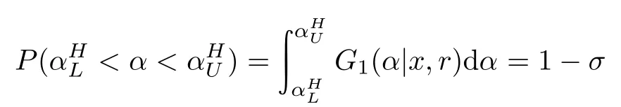
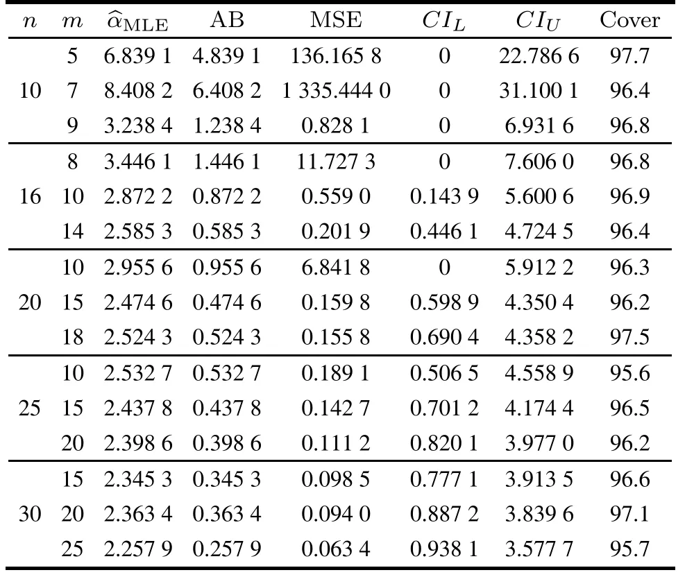
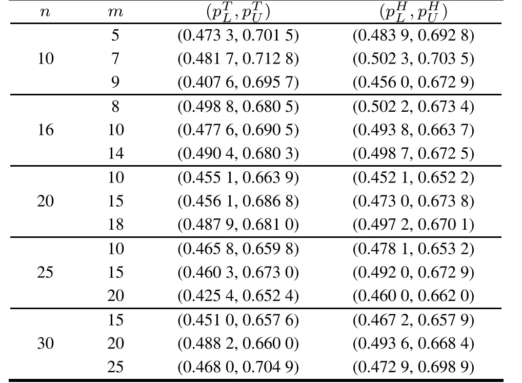
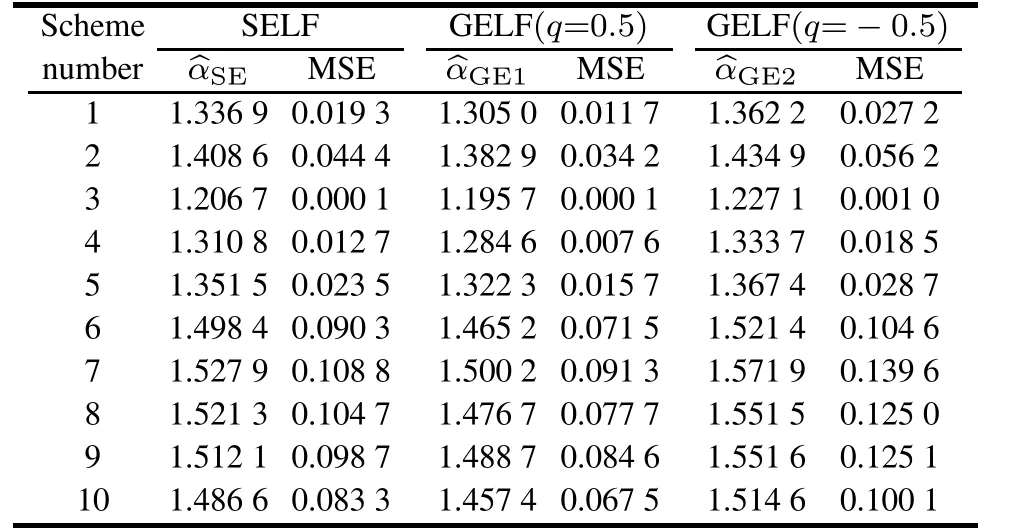
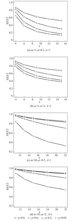
ProofSinceso 0

Whenα →0+,

and

Whenα →+∞,

and

Whenλ →0+,that isBi →0+,

Whenλ →+∞,that is,Bi →1-

However,analytic solutions ofandare not available through solving directly, so we need to apply a numerical technique,the Newton–Raphson method,to get the MLEs of them in the following sections.

According to the invariance property of the maximum likelihood estimation,(3)and(4),the MLEs of the two reliability indices are given by

In addition,sinceL2(p)only involves the parameterp,through maximizing log-likelihood function ofL2(p),it is easy to find that

3.2 Confidence intervals

In this subsection,we derive the 100(1-τ)%confidence intervals of the parameters.The unknown parameters can be denoted asβ=(β1,β2,β3)=(α,λ,p).

The Fisher information matrix provides a summary of the amount of information in the data we are interested in,which we can apply to obtaining the asymptotic variances and convariances of the MLEs. The information matrixI(β) for a differentiable log-likelihood function is given byIij= E(-2lnL/ βi βj) (i,j= 1,2,3). However,the above expectations are not easy to get. Therefore,the observed Fisher information matrix can be utilized instead.The elements of the observed matrix are given respectively as follows:

where

Lawless et al. [21] pointed out the asymptotic distribution theory of maximum likelihood estimation: using the large sample approximation, the asymptotic distribution of the MLEis, whereI-1(β) is the inverse of the observed information matrix ofβ=(α,λ,p),taking the following form:

4.Bayesian estimators

This section is devoted to Bayesian estimators of the parameters including the point and interval estimation. We consider symmetric and asymmetric loss functions (LFs)in the process of estimation. The interval estimation subsection discusses two special credible intervals: the twosided Bayes probability interval and the highest posterior density credible interval.

4.1 Point estimation

We have already known from(11)that

Becauseα,λandpare all unknown parameters,we can take the piecewise independent priors into account.Choose the Gamma distribution forα,the generalized exponential power distribution forλand the Beta distribution forpwith respective prior PDFs as follows:

Therefore,the joint prior PDF is

After that,the joint posterior PDF ofα,λandpcan be calculated by the following formula:

Combining the likelihood given in (17) with the joint prior PDF given in(18),it is easy to know that

Denote

Thus, the marginal posterior PDFs ofα,λandpare given by

and the conditional posterior PDFs ofαandλare

Because symmetric LFs are not always applicable in industrial production inference, we select symmetric and asymmetric LFs respectively in order to fully consider Bayesian estimation. A common symmetric loss function is squared error loss function(SELF) which is defined aswhereηis the parameter to be estimated andηis the estimator.Under the SELF,the Bayesian estimator and the posterior risk are the posterior mean and variance respectively.

As for asymmetric LFs, the general entropy loss function (GELF) is chosen, which has the following expression:

In this case,the Bayesian estimator can be obtained as

and the posterior risk(PR)is

Hence, after we get the posterior PDFs, the Bayesian estimator and the PR ofα,λandpunder different LFs are given by

whereφstands forα,λorp(i=1,2,3)respectively.

Specially,the Bayesian estimator and the posterior risk ofpunder the SELF can be calculated directly as follows:

Similarly,based on different LFs,the Bayesian estimation of reliability characteristics can be obtained as

whereSh(x)means the survival function or hazard function or any other reliability characteristics related toαandλ.

4.2 Credible intervals

4.2.1 Two-sided Bayes probability interval

Based on the posterior PDF of the parameterαgiven in(21),a symmetric 100(1-σ)%two-sided Bayes probability interval ofα,(),can be obtained by solving the following simultaneous equations:

and

In a similar way, according to (22)and (23), the equations for the two-sided Bayes probability interval ofλandp,denoted by()and()respectively,are written as follows:

and

4.2.2 HPD credible interval

As the posterior PDFsandof the parametersα,λandpare unimodal,we can find a credible interval meeting that the probability of the interval is 1-σand the posterior functional values are equal at the upper and lower bound of the interval.

Based on the posterior PDF of the parameterαgiven in (21), its 100(1-σ)% highest posterior density (HPD)credible interval()can be obtained from the simultaneous solution of the following two equations:

and

Similarly,using(22)and(23),the HPD credible intervalandofλandpare respectively derived by solving the equations as follows:

and

5.Monte Carlo simulation study

In this section, we carry out Monte Carlo simulations to evaluate the performance of the estimation methods proposed in previous sections. Under progressively Type-II censoring with binomial removals, without loss of generality,we consider different combinations fornandmand take the parametersp=0.5,α=2,λ=1.

5.1 MLE simulation

The MLE simulation process is conducted according to the following steps.

Step 1For a givennandm, generate a random removal planr= (r1,r2,...,rm) following the binomial distribution with the parameterp=0.5.

Step 2For the samenandm, generate a progressively Type-II censoring sample with the binomial removalx= (x1:m:n,x2:m:n,...,xm:m:n) following the GR distribution withα= 2,λ= 1, and is removed randomly according torgenerated in Step 1. The method to generate the progressively Type-II censoring sample was derived and presented in[22].

Step 3Calculate the MLEs ofα,λandpusing the method mentioned in Section 3,and obtain the point estimates,the average bias,mean squared error and 95%confidence intervals.

Step 4Repeat Steps 1–3 for 10 000 times,then we can get the results for the givennandm:the average bias (AB), mean squared error (MSE), 95%confidence interval(CIL,CIU) and the confidence interval coverage(Cover).

Step 5Choose differentnandmand conduct Steps 1–4 respectively. The final MLE results are tabulated in Table 2–Table 4.

Table 2 MLE of p for different(n,m)

As we can see from Table 2–Table 4,the MLEsandare close to the true valuesp= 0.5,α= 2,λ= 1.Especially forλandp,the ABs and MSEs are both small. However, the estimation error ofαis relatively large when the censored sample size is very small.In addition,forαandλ,with the increase ofnandm,the MSE decreases gradually;for the samen,whenmis closer ton,the MSE is smaller.While forp,the opposite is true.Whenmis closer ton,due to less censoring information,the estimation is more inaccurate. In term of confidence intervals,the intervals can cover the true values of the parameters,and the coverage is close to 95%.The method to obtain MLEs proposed above is effective.Because of the invariance property of MLE, we can know that the MLE results of reliability indices will not be bad as the effect of parameter estimation is relatively good,so we will not reiterate them here.

Table 3 MLE of α for different(n,m)

Table 4 MLE of λ for different(n,m)

5.2 Bayesian estimation simulation

In Bayesian estimation,the situation is more complicated,which involves the selection of appropriate hyperparameters of prior distribution and LF. It is a good method to find suitable hyperparameters by regarding the mean and variance of prior distribution as the selection criteria.

In our selected priorsg1(α),g2(λ) andg3(p), we already knowand E(p) =c/(c+d), then according to the MLEs we fix the means are 2, 1, 0.5 respectively,choosea2= 2.5,b2= 1,c=d= 1.Owing to the imprecise MLE results ofα, we focus on its hyperparameters selection. We take the variance of prior distribution1,4 respectively,that is,a1=8,b1=4 ora1=4,b1=2 ora1=1,b1=1/2.

The Markov chain Monte Carlo (MCMC) method is used to obtain Bayesian estimation of parameters and reliability indices.One of the attractive methods of constructing an MCMC chain is the Metropolis-Hastings(MH)algorithm under Gibbs sampling procedure, through which we can get the posterior sample of(α,λ,p).

We make use of the method in[22]to generate censored samples,and then iterate 10 000 times in the MH algorithm under Gibbs sampling procedure by taking the first 1 000 times as the burn-in period,where the proposal density is normal distribution. After obtaining the simulated posterior samples, the Bayesian integral can be approximated by the sample mean and then we obtain the corresponding Bayesian estimation based on LFs. The whole process is repeated 500 times and the final Bayesian estimation results ofα,λandpunder different posterior variances ofα(var) (that is, different hyperparameters) and different LFs(SELF and GELF(q=±0.5)),consisting of the AB,MSE,PR,are presented in Table 5–Table 7 respectively.It is noteworthy that the Bayesian estimator ofpis independent of the hyperparametersa1andb1in the light of the posterior distribution ofp.

From Table 5–Table 7,it can be seen that the Bayesian estimation results are extremely good,the bias and MSEs are very small, close to the true values. The selection of hyperparameters affects the estimation results ofαandλ.The larger the prior variance ofαis,the higher the estimation deviation will be,and it sheds more obvious influence on the estimation ofα.Besides,the estimation ofαandλare more accurate when the sample size is relatively large.However,forp, the more units removed from the sample,that is, the smaller the censored sample size is, the better the estimation effect will be.From the perspective of PR,the risk of the two cases of GELF are approximately equal,and are both smaller than that of the SELF.

Table 5 Bayesian estimation of α for different hyperparameters and different LFs

Table 6 Bayesian estimation of λ for different hyperparameters and different LFs

In order to compare the accuracy of the estimation, we draw the MSE plots for each parameter separately using the estimation under different LFs when the prior variance ofαis 4 (horizontal ordinate: 1–15 represents different(n,m)schemes respectively),as shown in Fig.3.

Based on the MSE figures we can draw the following conclusions.

(i)Forα,the best estimation results are obtained under the SELF.

(ii)Forλ,under the SELF and the GELF(q=0.5),the estimation results are relatively good.

(iii)Forp,the best estimation results are obtained under the GELF(q=-0.5).

The Bayesian 95% credible intervals of parameters whena1= 8,b1= 4,a2= 2.5,b2= 1,c=d= 1 are given in Table 8 and Table 9.The credible intervals can cover the true parameter values and the length of HPD intervals is shorter compared with the two-sided Bayes probability intervals.Then we choose the SELF to estimate the reliability characteristics because the reliability indices are dependent on parametersαandλwhich can be better estimated using the SELF.The Bayesian estimators of reliability characteristics are obtained in Table 10.

Table 8 Bayesian credible intervals of α and λ for different(n,m)

Table 9 Bayesian credible intervals of p for different(n,m)

Table 10 Bayesian estimate of reliability characteristics

6.Real data analysis

In this section, we analyze a practical industrial case: the deep-groove ball bearing data, and the observations are the number of million revolutions before failure for each of the 23 ball bearings. The complete sample is given by(17.88 28.92 33.00 41.52 42.12 45.60 48.80 51.84 51.96 54.12 55.56 67.80 68.64 68.64 68.88 84.12 93.12 98.64 105.12 105.84 127.92 128.04 173.40).

This dataset was reported by[21]originally.Lieblein et al.[23]also used it as an example to conduct statistical investigation.In addition, Meintanis et al. indicated in [17]that the GR distribution could fit the dataset very well.

To show that this dataset follows the GR distribution,the results of the Kolmogorov-Smirnov(KS)test and the Chisquare test are summarized in Table 11. Fig. 4 draws the comparison plots between the observation value and fitted function for ball bearing data.

Table 11 Statistic and p value of KS and Chi-square test

It can be seen from Fig.4 that the empirical and the fitted distribution are close to each other as the scatter points surround the straight line(Fig.4(a))and the maximum distance between the two curves marked by the red dots is 0.157 04(Fig.4(b)).According to KS and Chi-square tests results in Table 11,pvalues are much larger than 0.05,so we believe that the GR distribution provides a good fit to this dataset.The MLEs of the parameters based on the ball bearing data are determined to beα= 1.20 andλ= 0.01 respectively.

Fig.4 Comparisons between observation value and fitted function

Here we employ the ball bearing dataset to consider the statistical inference for the GR distribution under progressively Type-II censoring with binomial removals.

We take the effective sample sizem= 12.Meanwhile,takep= 0.05, 0.1–0.9 respectively to generate ten random removal schemes.We will carry out the progressively Type-II censoring experiments with binomial removals and derive the MLEs and Bayesian estimators of parameters by taking advantage of various schemes respectively, and compare the performance of the estimates based on the MSEs in the end. The ten random removal schemes can be seen in Table 12.

Table 12 Random removal schemes

Table 13 and Table 14 present the MLE analysis results.

Table 13 MLE of α for ball bearing data under different schemes

Table 14 MLE of λ for ball bearing data under different schemes

From the MLE results, we select the hyperparametera1= 2.88,b1= 2.4,a2= 1.5,b2= 10. Table 15 and Table 16 present the Bayes analysis results under different LFs.

Table 15 Bayesian estimation of α for ball bearing data under different schemes

Table 16 Bayesian estimation of λ for ball bearing data under different schemes

From Table 14 and Table 16,we can conclude that,the change in the value of the binomial parameterp,or different LFs has little effects on the estimates ofλ.The MSEs are all small(the magnitude of them is 10-6)based on differentpvalues,meaning that the parameterλcan be well estimated.

In term of the estimation ofα,however,the accuracy of the MLE forαis related to the removal probabilityp(Table 13).It can be seen thatpin a range near 0.5 has a better estimate than the extreme values.From Table 15,one can see that Bayesian estimators ofαunder GELF (q= 0.5)possess the minimum MSE, which provides guidance for us to choose a reasonable random removal scheme to obtain a more accurate estimate.

The reliability characteristics are estimated under GELF(q=0.5),as shown in Fig.5.

Fig.5 Reliability characteristic estimation functions for ball bearing data

7.Expected experimentation time

In practice,the experimenters are concerned about the termination point of the censoring experiment, because the time and cost are directly related to it. Knowing the expected experimentation time may help them make choices better.

Under progressively Type-II censoring with binomial removals, suppose that the censored sample isX=(X1:m:n,X2:m:n,...,Xm:m:n) and the random removal scheme isR= (R1=r1,R2=r2,...,Rm=rm),then it is easy to know the termination point of the experiment isXm:m:n,so the expected experimentation time is just the expected value ofXm:m:n.In[6],the formula to calculate E(Xm:m:n|R=r) is misexpressed so that the correct result cannot be obtained. Thus, we use the formula from Balakrishnan et al.[24],and we have

where

Based on all the different random removal schemesR=(R1=r1,R2=r2,...,Rm=rm), E(Xm:m:n) can be calculated as follows:

whereg(r1)=n-m,g(ri)=n-m-r1-r2-···-ri-1(i=2,...,m-1),andP(R=r)can be obtained by(10).

After obtaining E(Xm:m:n), by settingr1= 0,r2=0,...,rm=0,and the sample sizem=nin(24),the expected experimentation time of the complete sample with the sample sizencan be expressed as

where

Plugging(25)and(26)into the following equation,the ratio of expected experiment time REET under progressively Type-II censoring with binomial removal is defined as follows:

REET can be regarded as the time efficiency of the experiment,obviously,which is a number between 0 and 1.The smaller REET is,the more efficient it is.With the purpose of analyzing how parametersα,λ,pand sample sizesmandnaffect REET,we takem=3,10,andp=0.05,0.3,0.6,0.9,to draw the REET plots.

As the properties of the GR distribution are greatly influenced by the parameterα, we chooseα=0.5 andα=2 to discuss respectively. For the scale parameterλ, nevertheless,we observe that it exerts little influence on REET through programming,so we just need to choose a certain value ofλ.In the following we takeλ=1.

The REET versus complete sample sizenplots for different values ofmandαwith various values ofp(m=3,10,p=0.05,0.3,0.6,0.9 andα=0.5,2)are depicted in Fig.6.

Fig.6 REET versus complete sample size n plot

It can be seen that for a largem,the ratio of the expected experiment time approaches 1 quite sharply,and when the parameterαchanges from 0.5 to 2,REET increases on the whole.In addition,REET is closely dependent on the binomial parameterp: for a fixednandm,with the increase ofp,REET are also increasing.

Whenp= 0.6, 0.9, the value of REET is relatively large. Especially form= 10, it approximately equals 1.In this case,althoughngoes up until 22,REET has little fluctuation.However,ifptakes the value less than 0.5 such as 0.3,0.05,the time ratio decreases greatly.

8.Conclusions

This paper has studied statistical inference for the GR distribution under progressively Type-II censoring with binomial removals. The MLE (Newton–Raphson method)and Bayesian procedure (MCMC method) of parameters as well as reliability characteristics are derived.

From the whole estimation process,we can see that the estimation results are good but the parameterαis more difficult to estimate compared withλandp.In MLE,with the increase ofnandm,the MSE decreases gradually.For the samen, whenmis closer ton, the MSE is smaller.While forp,the opposite is true.Due to less censoring information,the estimation is more inaccurate.In Bayesian estimation,the selection of hyperparameters and LFs will affect the final inference results. When the prior information matched with the true guess, that is, the prior distribution is close to the real parameter value, the Bayes estimators provide more precise estimates. In the aspect of LFs,through simulation we find that it is not the same for estimation of different parameters.Finally, through a real case,we get the parameter estimators and the image of the reliability estimator function,which illustrates that the proposed method is effective.

The expected experimentation time is also investigated.The results show that the removal probabilityphas a great influence on the ratio of expected experiment time REET.Consequently, in practice, we should take both the estimation error (such as MSE) and REET into account to choose the value ofpreasonably,so that we can carry out the experiment more efficiently and obtain accurate statistical inference results.