Remaining useful lifetime prediction for equipment based on nonlinear implicit degradation modeling

CAI Zhongyi,WANG Zezhou,CHEN Yunxiang, GUO Jiansheng,and XIANG Huachun

Equipment Management and UAV Engineering College,Air Force Engineering University,Xi’an 710051,China

Abstract: Nonlinearity and implicitness are common degradation features of the stochastic degradation equipment for prognostics.These features have an uncertain effect on the remaining useful life(RUL)prediction of the equipment.The current data-driven RUL prediction method has not systematically studied the nonlinear hidden degradation modeling and the RUL distribution function. This paper uses the nonlinear Wiener process to build a dual nonlinear implicit degradation model.Based on the historical measured data of similar equipment,the maximum likelihood estimation algorithm is used to estimate the fixed coefficients and the prior distribution of a random coefficient. Using the on-site measured data of the target equipment,the posterior distribution of a random coefficient and actual degradation state are step-by-step updated based on Bayesian inference and the extended Kalman filtering algorithm.The analytical form of the RUL distribution function is derived based on the first hitting time distribution. Combined with the two case studies, the proposed method is verified to have certain advantages over the existing methods in the accuracy of prediction.

Keywords: remaining useful life (RUL) prediction, Wiener process,dual nonlinearity,measurement error,individual difference.

1.Introduction

In engineering, the equipment is affected by factors such as its complex composition, workload, operating environment, random impact, etc., and its performance may be degrading, e.g., the fatigue crack increasing of aeroengine blades,the drift increasing of gyroscope in the flight control system, the capacity reducing of lithium battery,etc. We refer to such equipment that is subject to performance degradation due to the combination of internal stress and external environment in actual service,and may eventually evolve into failure as stochastic degradation equipment[1,2].

In the early performancedegradation stage,by obtaining various types of degradation characteristic quantity,evaluating the health status of equipment,predicting its remaining useful life (RUL) (that is, the operation time interval from current time to failure time)and taking valid maintenance measures accordingly,it is important to improve the operational safety of the large and important system[3,4].

Professor Pecht [5] of Maryland University divided the RUL prediction methods into three categories: the mechanism-based method, the data-driven method, and a fusion of the first two.Based on the indepth analysis of the failure mechanism, the mechanism-based method establishes the mechanism model of the equipment and predicts its RUL[6,7].However,the cost of establishing the mechanism model is too large and it is almost impossible to implement it,which makes the application limited.The datadriven approach uses the monitored performance degradation data of the equipment to predict its RUL, which can be subdivided into the artificial intelligence method and the statistical data-driven method [8]. The artificial intelligence method is to learn the evolution law of the degradation process of the equipment through machine learning,but this method can only push out the expectation value of the equipment’s RUL, which has a certain limitation[9,10]. Considering the random dynamics of the equipment workload and operating environment,it is usually assumed that the remaining life is a conditional random variable.Based on this assumption and the probability theory,the statistical data-driven method can accurately describe the dynamic behavior of the equipment degradation process and quantify the uncertainty of RUL prediction results by using statistical models or stochastic process models,which has become a hot research topic[11].

At present,the statistical data-driven RUL prediction research focuses on the following two aspects.

The first aspect is degradation modeling, which is mainly modeling the dynamic behavior of the equipment degradation process.Tang et al.[12],Son et al.[13]and Li et al. [14] all thought that stochastic processes can better describe the evolution law of the equipment degradation process.Common stochastic processes include the Wiener process, the Gamma process, and the Markov chain. The latter two mainly describe a strictly monotonic,irreversible degradation process [15], which do not match the nonmonotonic features prevalent in engineering. The linear Wiener process can better describe the non-monotonic degradation process with a linear trend[16],where the drift coefficient is a parameter used to describe the degradation rate and the diffusion coefficient is a parameter used to describe the time-varying uncertainty of the degradation process.Due to its good mathematical calculation characteristics,the linear Wiener process and its extended form have been widely used in the research of lots of electronic equipment degradation modeling and RUL prediction, such as laser generator [17], LED [18], lithium battery [19] and Gyro[20].

The operating conditions,loads,and operating environments of equipment may change over time,resulting in different degradation rates,which make the degradation process exhibit a nonlinear feature.For the nonlinear degradation feature, early research mainly uses the data transformation technology [21,22] to convert nonlinear degradation data into linear degradation data,but not all nonlinear data can be linearized [2]. Si et al. [23] first put forward a general nonlinear Wiener process and approximated the first hitting time (FHT) distribution of equipment, which has an important impact on solving the nonlinear degradation modeling problem. Based on his research, Zhang et al. [24,25] further proposed an age- and state-dependent nonlinear prognostic model,which can better characterize the dynamics and nonlinearity of the degradation process.Many similar model extensions and deformations have emerged[26].

Because the equipment is affected by external random impacts during the manufacturing and using stage,there is a certain individual degradation difference between similar equipment.This individual difference will have an uncertain effect on the RUL prediction. Model parameters that generally describe individual difference are called the random coefficient. Peng et al. [20] considered that individual difference was mainly affected by degradation rate parameters. Thus, the drift coefficient in the Wiener process was regarded as a normal random variable and a linear Wiener degradation model considering individual difference was established. The study considers that when describing the specific degradation feature of the target equipment, the random coefficient is a fixed value [27].Zhai et al.[28]and Huang et al.[29,30]assumed the drift coefficient of the Wiener process as a normal distribution.Wang et al. [31] regarded the drift coefficient as a partial normal random variable,but the scope of application needs further study.

Due to the influence of disturbance and measuring device, the measured degradation state of equipment inevitably carries the measurement error, and its degradation process presents implicitness [32]. This implicitness is featured by a linear or nonlinear random relationship between the equipment’s measured state and its actual degradation state. For the first time, Whitmore [33]considered the measurement error as a standard normal random variable and was independent of the variance term of drift coefficient and standard Brownian motion. Tang et al. [34]and Zheng et al.[35]established a nonlinear Wiener degradation model that considers the individual difference and measurement error simultaneously.Si et al.[36]and Zheng et al. [37] described the three-layer uncertainty of RUL prediction results by the diffusion coefficient,the variance term of drift coefficient and the measurement error,and established the corresponding nonlinear Wiener degradation model.However,these studies assumed linear random relationship between the measured state and its actual degradation state, and did not take into account the nonlinear random relationship that is common in engineering. Although modeling such relationship may increase the computational difficulty,it helps improve the prediction accuracy. Feng et al. [38] studied the nonlinear random relationship of the equipment degradation process,but ignored the influence of individual difference on the uncertainty of the degradation model.

Through analysis, the nonlinear features of the equipment’s degradation process mainly reflect in two aspects.One is the nonlinearity of the equipment’s actual degradation state with time. The other is the nonlinear random relationship between the equipment’s measured state and its actual degradation state.At present,there are not many research institutes in this area.

The other aspect is RUL prediction,which is mainly the implicit state updating and the RUL distribution derivation.Based on the prior estimation results of model parameters,the former uses the target equipment’s on-site measured data to update the implicit state online and obtains the posterior estimate of the hidden state by the Bayesian inference method or random filtering algorithm. Based on the FHT distribution,the latter mainly uses the full probability formula to derive the RUL distribution function considering the uncertainty of the implicit state estimation.

For the RUL prediction model considering implicitness,the implicit state only refers to the actual degradation state.Si et al.[39,40]established the linear state space equation of the target equipment at the current condition monitoring (CM) time, and updated the actual degradation state by the Kalman filtering (KF) algorithm. Feng et al. [38]established a nonlinear state space equation for the target equipment at the current CM time.The extended KF(EKF)algorithm was used to update the actual degradation state for the RUL distribution.

For the RUL prediction models considering individual difference and implicitness,the implicit state refers to the random coefficient and the actual degradation state. Tang et al. [34]and Cai et al. [41]used the Bayesian inference method to update only the posterior distribution of the random coefficient,but did not accurately estimate the current actual degradation state, which would reduce the prediction accuracy. Si et al [36] and Zheng et al [37] used the KF algorithm to update the random coefficient and actual degradation states for the RUL distribution,and the prediction accuracy is higher.

In this paper,the main contribution include: (i)the proposal of nonlinear implicit degradation model to describe the implicitness and dual nonlinearity of the degradation process; (ii) the proposal step-by-step updating algorithm of implicit state in RUL distribution to obtain its posterior distribution. The remaining sections are organized as follows.Section 2 uses the nonlinear Wiener process to establish a dual nonlinear implicit degradation model of the equipment.Section 3 uses the maximum likelihood estimation (MLE) algorithm to obtain the prior estimates of the model parameters.Section 4 step-by-step updates the implicit state based on Bayesian inference and the EKF algorithm,and obtains the posterior distribution of the random coefficient and the actual degradation state. Section 5 derives the analytical form of the RUL distribution function considering the estimation uncertainty of the implicit state based on the FHT distribution. Section 6 uses two case studies to verify the advantages of the proposed method.Section 7 presents the conclusions.

2.Degradation modeling

Assume that the degradation state of the equipment can be described by a nonlinear Wiener process as follows:

whereX(0)is the initial degradation value,without loss of generality, letX(0) = 0.λis the drift coefficient, which describes the individual difference of degradation process in similar equipment.σBis the diffusion coefficient.B(t)is the standard Brownian motion.Λ(t;ϑ) is a nonlinear function of timetwith an unknown parameter vectorϑ,which describes the degradation nonlinearity itself.

Assume that the equipment’s failure threshold is a fixed value,denoted asw, and its FHT is denoted asTand can be expressed as

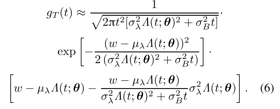
According to (1), the equipment’s FHT approximately obeys the inverse Gaussian distribution, and the probability density function(PDF)ofTunder a givenλis approximately deduced as

where

In order to describe the individual difference of the degradation process in similar equipment,λis generally considered to be a normal random variable, i.e.,We first introduce the following Lemma 1[23].

Lemma 1Ifλ ～N(μ,σ2),w1,w2,A,B ∈R, andC ∈R+,there is the following formula[23]:

Foraccording to(4)and Lemma 1,by using the full probability formula, the deduced PDF approximate expression is as follows:

with

There is a certain error in the direct measurement of the degradation process of the equipment.In order to describe the nonlinear random relationship between the direct measured state and the implicit actual degradation state,letY(t)denote the measured state,the actual degradation state is implicit and denoted asX(t).Then the relationship betweenY(t)andX(t)can be expressed as

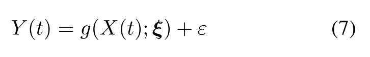
whereεdenotes the measurement error and is independent ofB(t),and assumeε ～N(0,σ2).g(X(t);ξ)is a nonlinear function withX(t)and contains an unknown parameter vector,denoted asξ.

Therefore, the dual nonlinearity in the above degradation model is mainly reflected in two aspects: one is to use a nonlinear function to describeX(t)witht. The other is to use a nonlinear function to describe the nonlinear random relationship betweenY(t)andX(t).The uncertainty in the above degradation model is mainly described by the three variance terms ofandσ2.

3.Prior parameter estimation

The modified EM algorithm was first proposed by Tang[42] in 2015 and applied to the parameters estimation of the linear Wiener degradation model with measurement error.Then,Cai et al.[4]applied this algorithm to the nonlinear Wiener degradation model,but this algorithm may lead to the case of non-converge.Therefore,this paper uses the MLE to estimate the prior parameters.

The unknown parameter set in the above degradation model is denoted as.Among themandσ2are called the fixed coefficients,which describe the common degradation feature among similar equipment;μλandis called the random coefficients, which describe the personality degradation feature of the target equipment.

It is assumed that the historical measured data of the same type ofNequipment are known. The CM time of theith equipment is denoted ast1,i,t2,i,...,tmi,i(i= 1,2,...,N);miis the number of CM times of theith equipment. The corresponding measured state is denoted asYi={Yi(t1,i),Yi(t2,i),...,Yi(tmi,i)}.The corresponding actual degradation state is denoted asXi={Xi(t1,i),Xi(t2,i),...,Xi(tmi,i)}. The measured state of theNequipment is denoted asY1:N={Y1,Y2,...,YN}and its corresponding actual degradation state is denoted asX1:N={X1,X2,...,XN}.The measured data of theith equipment attj,iare denoted asYi(tj,i) and the corresponding actual degradation data are denoted asXi(tj,i).The measured increment attj,iis denoted as ΔYi(tj,i) =Yi(tj,i)- Yi(tj-1,i)and the corresponding actual degradation increment is denoted as ΔXi(tj,i) =Xi(tj,i)- Xi(tj-1,i).Tj,i=Λ(tj,i;ϑ). ΔTj,i=Λ(tj,i;ϑ)- Λ(tj-1,i;ϑ). Let the measured increment of theith equipment be denoted as Δyi={ΔYi(t1,i),ΔYi(t2,i),...,ΔYi(tmi,i)}′. ΔTi={ΔT1,i,ΔT2,i,...,ΔTmi,i}′.

Because the nonlinear function form ofg(X(t);ξ)will cause difficulty for the construction of the likelihood function, the first-order Taylor development is generally used to approximate the linearization ofg(X(t);ξ)atX(0)as follows:

whereg′(X(0);ξ) represents the first derivative ofg(X(t);ξ) atX(0). Here, the nonlinear function form is assumed to beg(X(t);ξ) =βexp(X(t)), which is common in engineering and is taken as an example to illustrate the application of the above linearization.

According to (8), the following equation can be obtained.

According to the property of multivariate Wiener process, Δyiobeys the multivariate normal,and its expectation and covariance matrix are expressed as follows:

with

The log likelihood function ofY1:Nis

The MLE algorithm is used to estimate the parameter setΘ. First, let lnL(Y1:N) be zero for the first-order partial derivatives ofμλandrespectively:

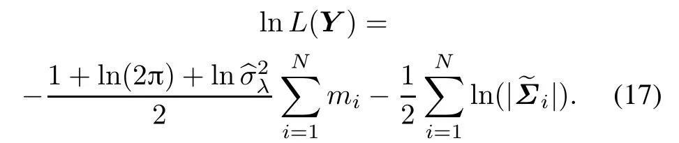
Maximizing(17)gives a maximum likelihood estimate forandThen, by substituting the estimates into(15)and(16),the priori estimates ofμλandcan be obtained.

4.Implicit state updating

The measured state of the target equipment at timetkis denoted asY1:k= (Y(t1),Y(t2),...,Y(tk)), and the corresponding actual degradation state is denoted asX1:k= (X(t1),X(t2),...,X(tk)). Let ΔTk=and ΔYk=Y(tk)-Y(tk-1).At this time,the drift coefficient is denoted asλkand the actual degradation state is denoted asX(tk). Both of them are the implicit states that need to be estimated fromY1:k.

Considering that the correlation between the posterior estimates ofλkandX(tk) has little effect in engineering practice,it can generally be considered that they are independent of each other.The updating of the implicit states is divided in two steps:firstly,the Bayesian inference method is used to updateλk;then the EKF algorithm is used to updateX(tk).

(i)λk

with

Equations(18)and(19)can solve the posterior distribution ofλkattk,expressed as

(ii)X(tk)

The state space equation is used to describe the measured state of the target equipment attkas follows:

whereεkis the measurement error atand{εk}k≥1are independent of each other.

Since the above state space equation is nonlinear withX(t), before the EKF algorithm is adopted,the linearization ofg(X(tk);ξ)atis performed as follows:

First,define the estimates of expectation and variance ofX(tk)based onY1:kas

Then, define the expectation and variance of the onestep prediction at this time:

Finally, the iterative estimation ofX(tk) in (20) is divided into two parts: prediction and updating.

Prediction

whereμλ,k-1is obtained by(18).

Updating

By step-by-step performing the above prediction and updating, the posterior distribution ofX(tk) attkcan be solved, which is expressed as

5.RUL distribution derivation

The equipment’s RUL attkis denoted asLk. The degradation trend of the equipment attkcan be represented byZ(lk)=X(lk+tk)-X(tk),thenLkcan be converted to the time when{Z(lk),lk≥0}first hits the new threshold,denoted aswk=w-X(tk). From (3), the approximate expression of PDF ofLkunder the givenλkandX(tk)is deduced as

whereϕ(lk)=Λ(lk+tk;ϑ)-Λ(tk;ϑ).

The PDF ofLkunder givenλk,X(tk)andY1:kis denoted as. According to the Markov property of the Brownian motion, we can obtain the following equation:

By using the full probability formula, the PDF ofLkunder the givenY1:kattkcan be deduced as

To solve the complete expression of the above equation,we introduce Lemma 2[34].

Lemma 2IfR, andC ∈R+, there is the following formula:

According to (27)–(29), it can be seen that the PDF approximate expression ofLkunder the givenY1:kis deduced as

The above equation considers the influence of the estimation uncertainty ofλkandX(tk)on the RUL distribution of a class of equipment,and can reflect the personality feature of the RUL prediction of the target equipment.The flowchart of the proposed RUL prediction method in this paper is shown in Fig.1.

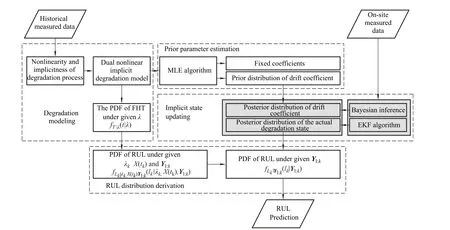
Fig.1 Flowchart of the proposed RUL prediction method

6.Case studies

6.1 Simulation data study

A numerical simulation example is exhibited by the Monte Carlo method to verify the correctness and advantages of the proposed method.

Without loss of generality,let.According to [38,43], we set the initial values of the simulation parameters asb= 1.5,β= 0.02,2= 0.09,= 0.062 5. Five sets of the simulated measurement data with measurement error are shown in Fig.2.

Fig.2 Five sets of simulated measurement data

The implicit degradation modeling method considering dual nonlinearity proposed in this paper is denoted as M1.The nonlinear implicit degradation modeling method considering only the nonlinearity of the actual degradation state itself (wherebis 1) is recorded as M2. The implicit degradation modeling method considering only the nonlinearity between the measured state and the actual degradation state proposed by Tang et al.[34]is denoted as M3.

The Akashi information criterion(AIC) is used to evaluate the model fitting accuracy. The mean square error(MSE) and total MSE (TMSE) are used to measure the model estimation accuracy.The specific formula is

wherepis the number of unknown parameters; lnL(Θ)represents the value of log likelihood function.

whereis the actual value of the remaining life attk;is the corresponding estimate values of PDF of the RUL.

whereKis the CM number.

(i)Prior parameter estimates

The five sets of measured data in Fig.2 are used as historical measured data of similar equipment.The MLE algorithm is used to obtain the prior parameter estimates in the degradation model.The results are shown in Table 1.

Table 1 Prior parameter estimates by M1,M2 and M3

It can be seen from Table 1 that the AICs and TMSEs of M1 are the smallest and the three variance terms are the smallest,which indicates that M1 has the smallest estimation error and the highest model fitting accuracy. This is because M1 simultaneously models the uncertainty of dual nonlinearity on the degradation model, which can better describe the nonlinear evolution of the equipment’s implicit degradation process, while M2 ignores the nonlinearity of the actual degradation state itself, which has the uncertain effect on equipment’degradation process.M3 ignores the uncertain effect of the nonlinear random relationship between the measured state and the actual degradation state on the equipment’s degradation process. Therefore,the model fitting accuracy of M2 and M3 is relatively lower, which will lead to a large deviation between the proposed implicit degradation model of equipment and its degradation process.

(ii)RUL prediction

Feng et al.[38]also established a dual nonlinear implicit degradation model, but the research background only has single equipment’s on-site measured data without historical measured data, so only the actual degradation state is updated in implicit state updating.Therefore,his research is significantly different from the background of this paper.

In order to further verify the advantages of the proposed synchronous updating of the drift coefficient and the actual degradation state.Based on the dual nonlinear implicit degradation model, the RUL prediction model proposed in this paper is still denoted as M1. The RUL prediction model only updating the actual degradation state proposed by Feng et al.[38]is denoted as M4.The RUL prediction model which only updates the drift coefficient proposed by Cai et al.[4]is denoted as M5.

Fig.3 shows the measured data of the target equipment and its actual degradation data by simulation.It is known that the target equipment has an actual degradation value of 13.00 at the end of CM time (at 5 h). Assume that the failure threshold for this type of equipment is 12.99,then the equipment is just to be a failure at 5 h.

Fig.3 Simulated measurement path and actual degradation path of target equipment

The PDFs of the RUL under M1, M4 and M5, and the PDFs of the RUL at 4.5 h under M1, M4, and M5 are shown in Fig.4 and Fig.5 respectively.

Fig.4 PDFs of RUL under M1,M4 and M5

Fig.5 PDFs of RUL at 4.5 h under M1,M4 and M5

It can be seen that the PDFs of RUL by M1,M4 and M5 can cover the actual values of RUL of the target equipment,but the PDFs by M1 is narrower than those of M4 and M5,which indicates that the model prediction accuracy of M1 is better than those of M4 and M5. This is because M1 uses the on-site measured data of the target equipment to synchronously update the posterior distribution of the drift coefficient and the current actual degradation state,so that the PDFs of the RUL are more in line with the personality features of target equipment.

However, M4 only updates the current actual degradation state,ignoring the uncertainty effect of the drift coefficient estimates on the RUL distribution.M5 only updates the drift coefficient, ignoring the uncertainty effect of the actual degradation state estimates on the RUL distribution.Both M4 and M5 will increase the uncertainty of the RUL prediction results and reduce the prediction accuracy.

At the same time, the 95% confidence interval (CI) of RUL by M1, M4 and M5 at each CM time is shown in Fig.6.

Fig.6 The 95%CI of RUL by M1,M4 and M5

It can be seen from Fig.6 that the 95%CI of the RUL by M1,M4 and M5 can cover the actual values of the RUL of the target equipment,but it is clear that the CI of the RUL by M1 is narrower than that of M4 and M5, which helps reduce the uncertainty of RUL prediction results and can better adapt to the personality prediction demand of the target equipment, and further demonstrate that the model prediction accuracy of M1 is better than that of M4 and M5.

Further,the MSEs of M1,M4,and M5 at each CM time are calculated and shown in Fig.7.

Fig.7 Comparison of MSEs of M1,M4 and M5

It can be seen that the MSEs of M1 are always lower than those of M4 and M5,indicating that the RUL estimation error of M1 is less than that of M4 and M5.As the CM time prolongs,the MSEs of M1,M4 and M5 gradually become small.This is because as the on-site measured data of the target equipment increase,the posterior distribution of the implicit states is step-by-step updated,so that the RUL prediction accuracy of the equipment is further improved.This can be confirmed by the gradually narrowing PDFs of the RUL by M1,M4 and M5 in Fig.4.

6.2 Milling data study

Milling cutter is an important component of milling machine and will degrade in use. The frank ware VB of the milling cutter is generally used as a key performance degradation feature.This paper uses the actual milling data set provided by NASA [44] for a case analysis. The four sets of milling data are shown in Fig.8 by setting the cutting depth to 0.75 mm and the cutting material to be cast iron.

Fig.8 Four sets of milling degradation data

According to Fig.8,the degradation path of the milling cutter shows obvious nonlinear characteristics.Therefore,we use M1 proposed by this paper to build the implicit degradation model and use MLE to obtain the estimates of the unknown parameters asuλ= 0.032 8,= 0.009 2,b= 1.26,β= 0.035 0,= 0.000 2;σ2= 0.001 6.Furthermore,the Kolmogorov-Smirnov(K-S)test is used to do distribution hypothesis test for Δyiand the result shows that Δyiobeys the normal distribution where thePvalue is 0.85, which means the degradation process of the milling cutter obeys the Wiener process approximately.Therefore,the degradation path of the milling cutter shows dual nonlinearity,which matches the proposed model.

Then,we use the milling data of Sample1 to verify the accuracy of the proposed RUL model.It is known that the RUL actual value of Sample1 at 60 times is 12.The PDFs of the RUL at 60 times by M1, M4 and M5 are shown in Fig.9.

Fig.9 PDFs of RUL at 60 times

It can be seen that the PDFs of the RUL at 60 times by M1,M4 and M5 can cover the actual values of Sample1’s RUL,but the PDF by M1 is narrower than that of M4 and M5,which indicates that the model prediction accuracy of M1 is better than M4 and M5,which is in accordance with the simulation data study and further verifies the accuracy of the proposed RUL model.

7.Conclusions

First, this paper proposes a dual nonlinear implicit degradation modeling method, which can accurately describe the implicitness and dual nonlinearity of equipment’s degradation process. Second, using the on-site measured data of the target equipment, the posterior distribution of the drift coefficient and the actual degradation state are updated synchronously based on Bayesian inference and the EKF algorithm,which meets the individual prediction demand of the RUL for the target equipment and improves its prediction accuracy. Finally, combined with two case studies, by comparing the AICs and TMSEs of different degradation models, the dual nonlinear implicit degradation modeling method proposed by this paper has certain advantages on model fitting accuracy and parameter estimation error.By comparing the PDFs,CI and MSEs of different RUL prediction models,the RUL prediction method considering the estimation uncertainty of the drift coefficient and the true degradation state simultaneously proposed by this paper has a certain advantage on prediction accuracy,which would have good engineering application values.

In this paper, the forms of the dual nonlinear function are simple and common, which is in accordance with the degradation features of the specific equipment, like the milling cutter.In order to extend the application field of the proposed model,more forms of the dual nonlinear function will be studied in future research.