Numerical Treatment for a Class of Partial Integro-Differential Equations with a Weakly Singular Kernel Using Chebyshev Wavelets
2019-10-16XUXiaoyong许小勇ZHOUFengying周凤英XIEYu谢宇
XU Xiaoyong(许小勇),ZHOU Fengying(周凤英),XIE Yu(谢宇)
(School of Science,East China University of Technology,Nanchang 330013,China)
Abstract: In this paper,a numerical method based on fourth kind Chebyshev wavelet collocation method is applied for solving a class of partial integro-differential equations(PIDEs)with a weakly singular kernel under three types of boundary conditions.Fractional integral formula of a single Chebyshev wavelet in the Riemann-Liouville sense is derived by means of shifted Chebyshev polynomials of the fourth kind.By implementing fractional integral formula and two-dimensional fourth kind Chebyhev wavelets together with collocation method,PIDEs with a weakly singular kernel are converted into system of algebraic equation.The convergence analysis of two-dimensional fourth kind Chebyhev wavelets is investigated.Some numerical examples are included for demonstrating the efficiency of the proposed method.
Key words: Partial integro-differential equation;Weakly singular kernel;Fourth kind Chebyshev wavelet;Collocation method;Fractional integral
1.Introduction
In science and engineering,many of the problems can be modeled as mathematical equations,including partial differential equations,integro-differential equations and partial integro-differential equations with weakly singular kernels and others.Recently,fourth-order problems have become the focus of many scholars.For example,airplane wings,bridge slabs,floor systems,and window glasses etc.are modeled by fourth-order partial differential equations.Many numerical methods are proposed for the fourth-order partial differential problems in the last few decades.[1−8]In the present work,we consider the following fourth-order partial integro-differential equations (PIDEs) with a weakly singular kernel subject to the initial condition


and the following three types of boundary conditions are considered as follows:
(I)
(II)
(III)
where 0<α<1 andpare constants.
Owing to the memory effect of integral term,it is difficult to design fast and accurate algorithms.Therefore,developing efficient numerical method for PIDEs with weakly singular kernel is still a challenge and has attracted much attention.
Many scholars have proposed different methods for partial differential equations with weakly singular kernel.Yanik and Fairweather[9]applied finite element methods to obtain the solution of a parabolic type integro-differential equations.In [10],Galerkin finite method is used to solve a parabolic integro-differential equation with a weakly singular kernel.TANG[11]solved a second-order partial integro-differential equations by finite difference method.LI and XU[12]adopted finite central difference and finite element approximation for the numerical solution of parabolic integro-differential equation.ZHANG et al.[13]proposed quintic B-spline collocation method for the numerical solution of fourth-order PIDEs with a weakly singular kernel.Also the quintic B-spline methods are used to solve time fractional fourth-order partial differential equations[14].In[15],FD-RBF method is proposed for solving PIDE with a weakly singular kernel.A compact difference scheme is presented for PIDEs with a weakly singular kernel in [16].Recently,quasi-wavelets numerical methods are proposed to solve PIDEs and the time-dependent fractional partial differential equation[17−18].
It is worth noting that the above methods adopted the finite difference schemes to approximate time variable.Spectral methods are widely used in seeking numerical solutions for different types of differential equations,owing to their excellent error properties and exponential rates of convergence for smooth problems.If the spectral method is used for space discretization then the finite difference schemes are used to deal with time variable,the accuracy of the numerical of smooth problems would be limited by the finite difference schemes.Wavelets,as another basis set and very well-localized functions,are considerably useful for solving differential and integral equations.According to the localization properties of wavelets,it can analyze the local characteristic of functions,which makes wavelet-based method be an effective tool in dealing with the sharp transitions caused by the singularities of the kernel.Methods based on Chebyshev wavelets have gained much attention during the last decade.It is well known that there are four kinds of Chebyshev wavelets[19].In the literature,there is a great concentration on the first and the second kinds of Chebyshev wavelets and their various uses in numerous applications.However,there are few articles that concentrate on the third and fourth kinds.
Inspired and motivated by the work mentioned above,the main purpose of this paper is to propose an effective method based on frouth kind Chebyshev wavelets method collocation,which is applied both in space and time directions to obtain numerical solution of fourthorder PIDE with a weakly singular kernel and further extend the application of Chebyshev wavelets.The rest of the paper is organized as follows.Section 2 describes some necessary definitions and preliminaries of calculus.Section 3 gives some properties of fourth kind Chebyshev wavelets and proves the convergence analysis of two-dimensional fourth kind Chebyshev wavelets.Section 4 is devoted to deriving the fractional integral of a single Cheyshev wavelet in the sense of Riemann-Liouville fractional integral.The proposed method is described for solving PIDEs in Section 5.In Section 6,the numerical results are presented.Finally,a brief conclusion is stated in Section 7.
2.Definitions and Preliminaries
In this section,we present some necessary definitions and preliminaries of the fractional calculus theory which will be used later.
Definition 2.1A real functionh(t),t>0,is said to be in the spaceCσ,σ∈R,if there is a real numberρwithρ>σsuch thath(t)=tρh0(t),whereh0(t)∈C[0,∞),andh(t)∈Cnσifh(n)(t)∈Cσ,n∈N.
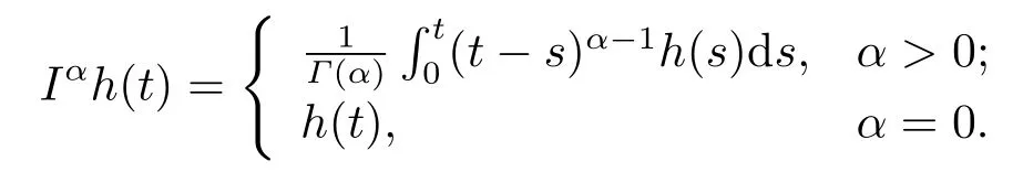
Definition 2.2The Riemann-Liouville fractional integral operatorIαof orderα(α≥0)for a functionh(t)∈Cσ(σ≥−1) is defined as in [20]
Definition 2.3The Caputo fractional derivative operatorDαof orderα(α≥0) for a functionh(t)∈Cn1is defined as in [20]
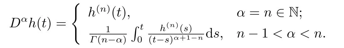
Some important properties of the operatorIαandDαare needed in this paper,we only mention the following properties
1)Iα1Iα2h(t)=Iα1+α2h(t) forα1,α2>0;
2)DαIαh(t)=h(t),DβIαh(t)=Iα−βh(t),α>β;
3)Dαtn=n≥⌈α⌉;Dαtn=0,n≥⌈α⌉,n∈N;
4)IαDαh(t)=h(t)−t >0,where we use the ceiling function⌈α⌉to denote the smallest integer than or equal toα.For more details about fractional calculus and its properties,see [20].
3.The Fourth Kind Chebyshev Wavelets and Their Properties
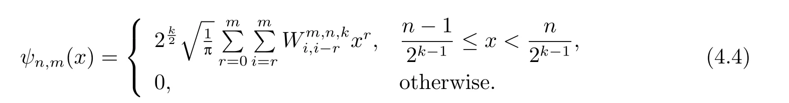
The fourth kind Chebyshev wavelets defined on the interval [0,1) has the following form wheren=1,2,3,···,2k−1and

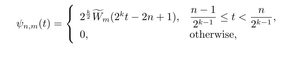
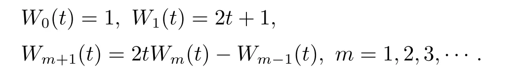
The coefficient in Eq.(3.1) is for orthonormality.HereWm(t) are the fourth kind Chebyshev polynomials of degreemwhich are orthogonal with respect to the weight functionω(t)=√on the interval [−1,1]and satisfy the following recursive formula:
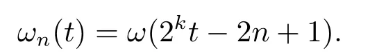
Note that when dealing with the fourth kind Chebyshev wavelets the weight function has to be dilated and translated as
A functionf(x)∈L2(R)defined on[0,1)may be expanded by the fourth kind Chebyshev wavelets as

where

in which2ω[0,1)denotes the inner product inL2ω[0,1).If the infinite series in Eq.(3.2) is truncated,then it can be written as
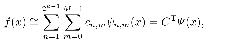
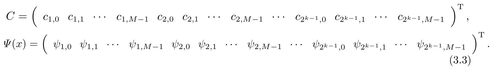
whereCandΨ(x) are 2k−1M ×1 matrices given by
The two-dimensional fourth kind Chebyshev wavelets of the fourth kind are defined as
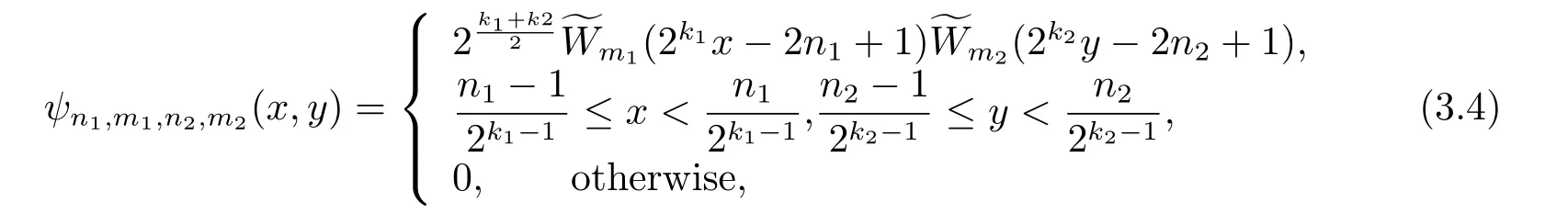
wheren1andn2are defined similaryly ton,k1andk2are any positive integers,m1andm2are the orders of fourth kind Chebyshev polynomials andψn1,m1,n2,m2(x,y) forms a basis forL2ω([0,1)×[0,1)).A functionµ(x,y) defined on [0,1)×[0,1) can be expanded by twodimensional fourth kind Chebyshev wavelets as follows

If the infinite series in Eq.(3.5) is truncated,then it can be written as
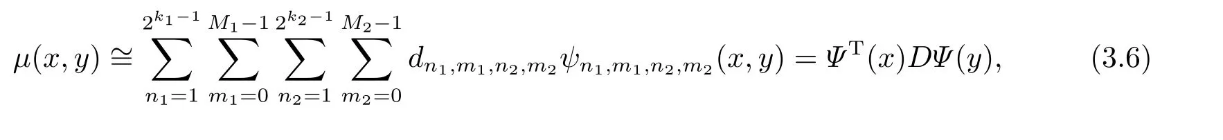
whereΨ(x) andΨ(t) are 2k1−1M1×1 and 2k2−1M2×1 matrices and are defined in (3.3).Moreover,Dis 2k1−1M1×2k2−1M2matrix and its elements can be calculated from the formula

wheren1=1,···,2k1−1,m1=0,···,M1−1,n2=1,···,2k2−1,m2=0,···,M2−1.In the calculation,we usually takek=k1=k2andM=M1=M2.
We investigate the convergence analysis of two-dimensional fourth kind Chebyhev wavelets in the following theorem.
Theorem 3.1Suppose thatµ(x,y)∈L2(R2)is a continuous function defined on[0,1)×[0,1),and satisfiesfor some positive constantB.Then the series
converges toµ(x,y),wheredn1,m1,n2,m2=
Proof

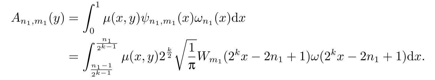
Let 2kx−2n1+1=tand dx=√dt.It follows

By puttingt=cosθ,together with the definition of the fourth kind Chebyshev polynomial,we get
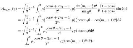
Applying the integration by parts,we have
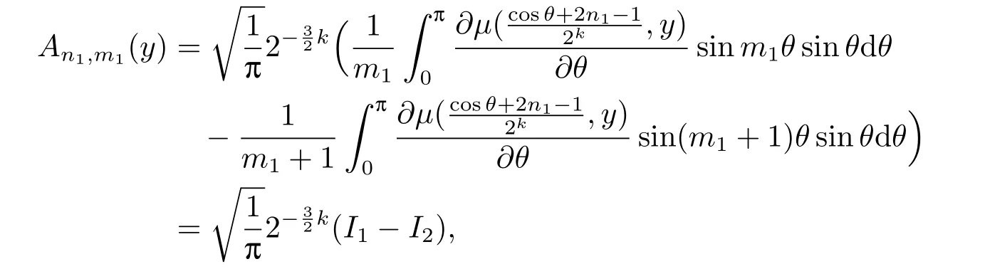
where
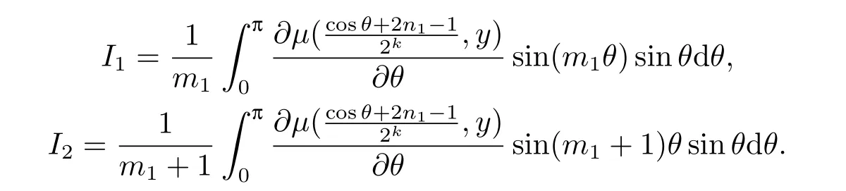
Using the integration by parts again,we get
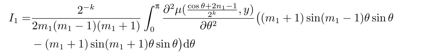
and
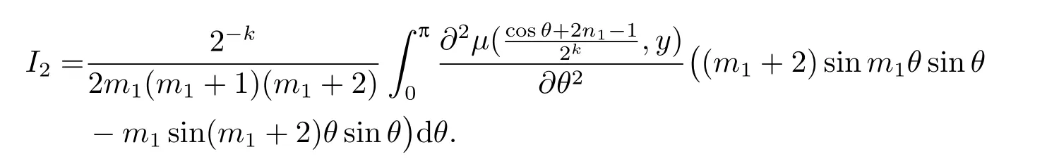
Therefore

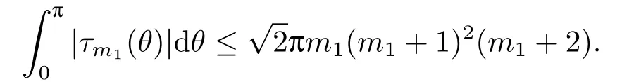
whereτm1(θ)=m1(m1+1)2(m1+2)sin(m1−1)θsinθ−m1(m1−1)(m1+1)(m1+2)sin(m1+1)θsinθ−m1(m1−1)(m1+1)(m1+2)sinm1θsinθ+m21(m1−1)(m1+1)sin(m1+2)θsinθ.
So,form1>1,m2>1,

A simple computation shows that
Hence,form1>1 andm2>1,we have


sincen1≤2k−1andn2≤2k−1.Form1>1 andm2=1,

So

Similarly,form1=1 andm2>1,
form1>1 andm2=0,

form1=0 andm2>1,
form1=1 andm2=1,
form1=1,0 andm2=0,1
Hence,by relations (3.7)-(3.13),the seriesconverges toµ(x,y) uniformly.The proof is completed.
4.The Fractional Integral of a Single Chebyshev Wavelet
In Section 5,multiple integrals onψn,m(x) will be performed from 0 tox.In this section,fractional integral formula of a single Chebyshev wavelet in the Riemann-Liouville sense is derived by means of shifted Chebyshev polynomials of the fourth kind,which plays an important role in solving PIDEs with weakly singular kernels.
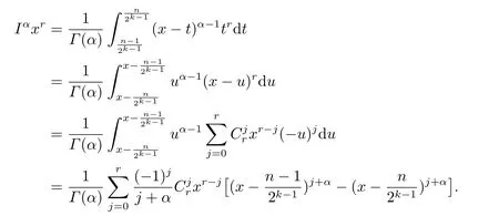
Theorem 4.1The fractional integral of a Chebyshev wavelet defined on the interval[0,1]with compact supportis given by
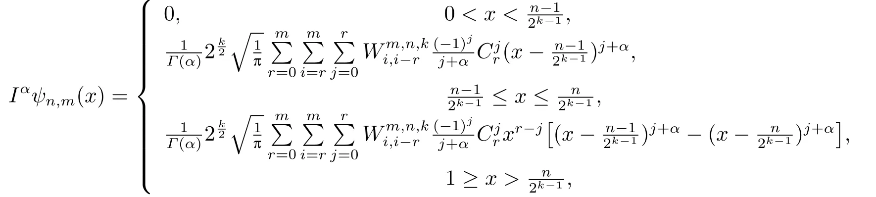
ProofThe analytical form of the shifted Chebyshev polynomials of the fourth kindW∗mof degreemis given by [19]

According to the relation betweenW∗m(x) andWm(x),it gives that
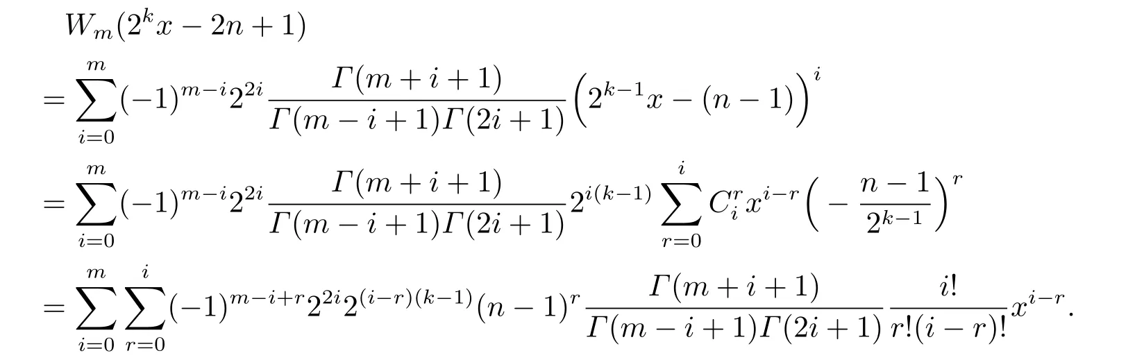
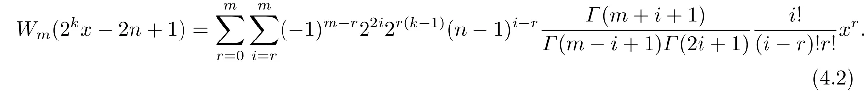
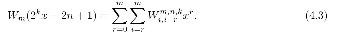
By interchanging the summation and substitutingi−rwithr,Wm(2kx−2n+1) can be written as
Therefore

In a similar way,whenx>,we have
Applying the Riemann-Liouville fractional integral of orderαwith respect toxonψn,m(x),we obtain
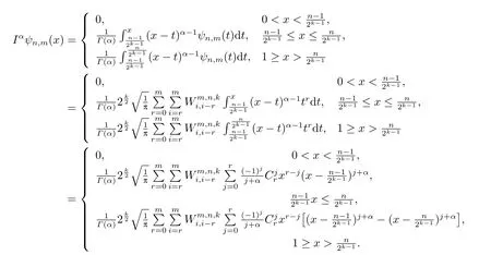
Thus,we have
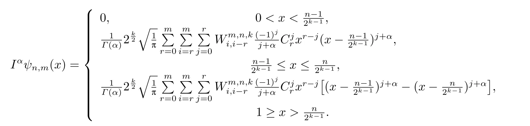
The proof is completed.
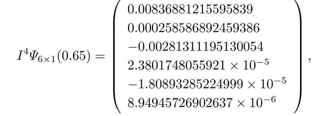
For example,in the case ofk=2,M=3,x=0.65,α=4,we obtain
5.Description of the Proposed Method
To solve the partial integro-differential equations given in (1.1) under the three conditions (I)-(III),first we assume that the mixed derivative of the solutionu(x,t) in (1.1) is approximated by Chebyshev wavelets as

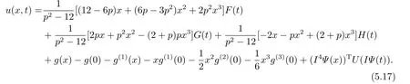
whereUis an unknown matrix which should be determined.By integrating(5.1)with respect totand combining the initial condition (1.2),we obtain:

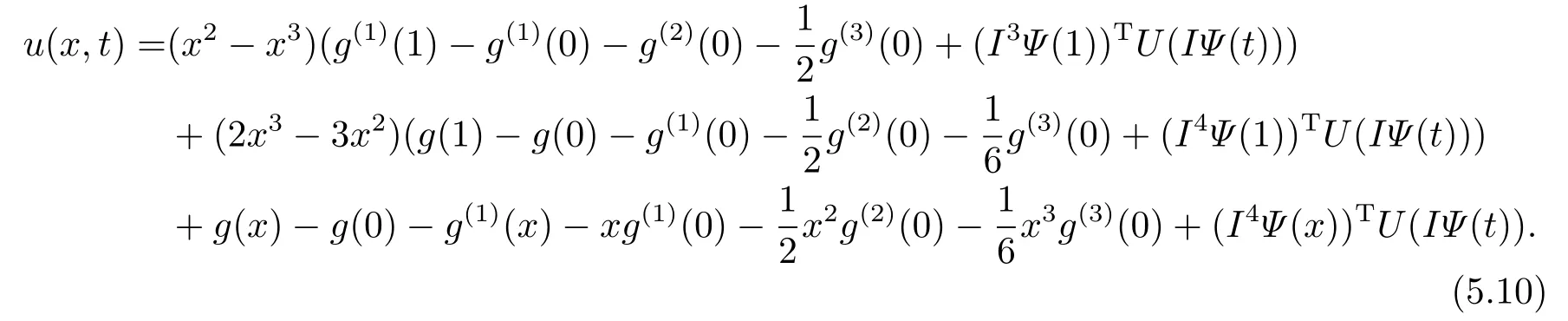
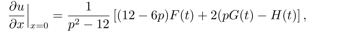
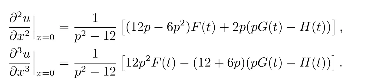
Also by integrating (5.2) four times with respect tox,we get the following equations
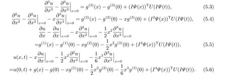
We introduce the following notations
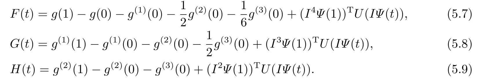
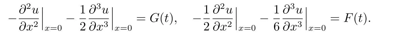
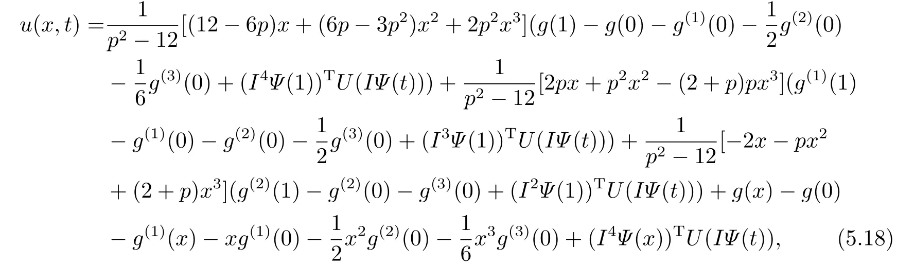
For the first type of boundary condition (I),by puttingx=1 into Eqs.(5.5),(5.6),we obtain a linear system ofwhich can be written as
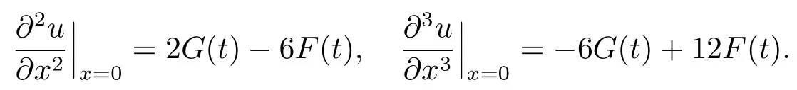

Therefore,we have
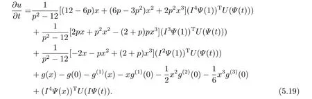
By applying the first order derivative with respect totonu(x,t),we have

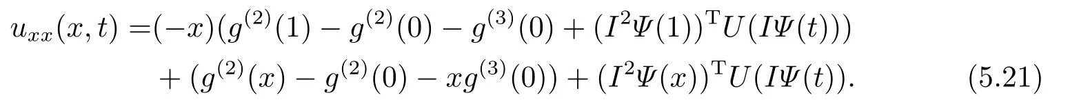
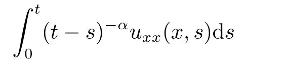
Next we calculate the integral term
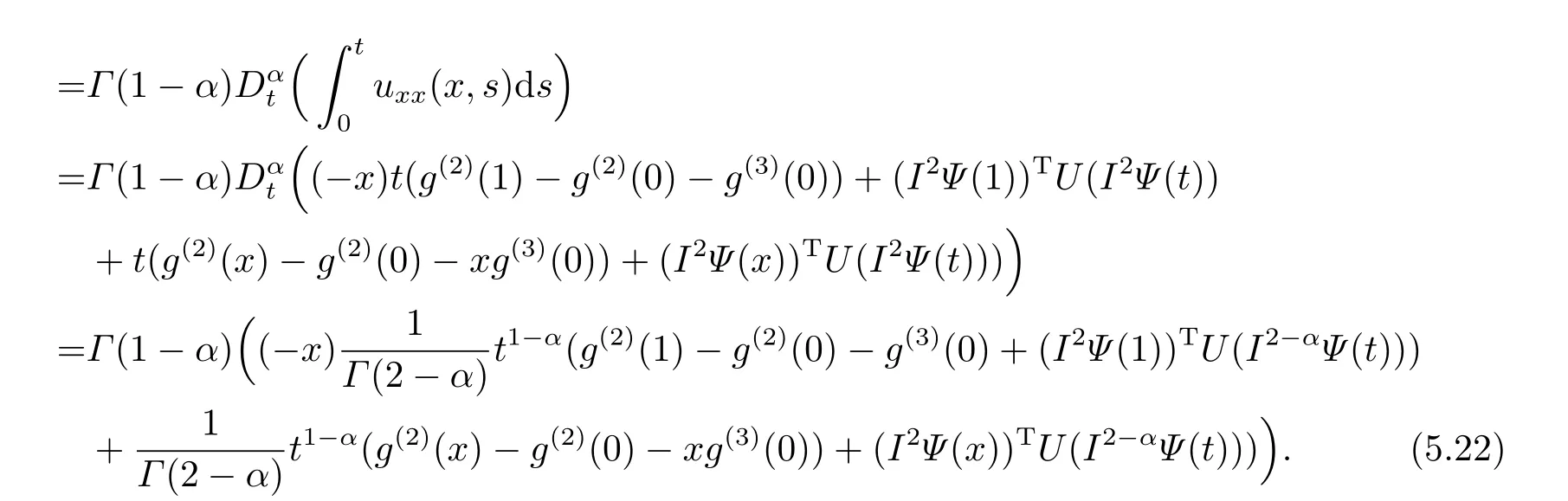
Note that

According the definition of fractional derivative in the Caputo sense,we have
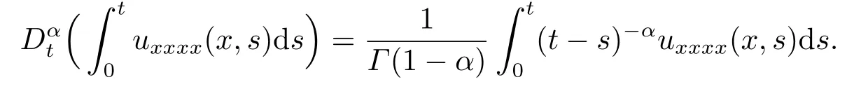
Therefore

In order to calculate the unknown matrixUin (5.1),the following collocation points are considered,

Substituting(5.11),(5.12)into Eq.(1.1)and substituting the collocation points into Eq.(1.1),we obtain the following linear system of algebraic equations:
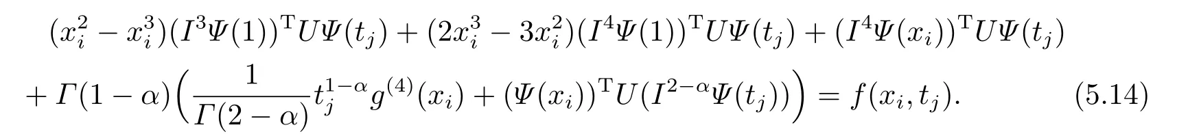
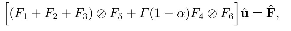
where
By solving this system and determiningU,we get the numerical solution of the problem by substitutingUinto (5.10).
In a similar way,we can deal with the problems under the other two types of boundary conditions.For simplicity,we also only give the derivation ofu(x,t)andunder the following two types of boundary conditions.
For the second type of boundary condition (II),by puttingx=1 into Eqs.(5.4),(5.6),we can easily getBy puttinginto(5.6) and combining the boundary condition,we obtain

and

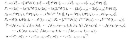
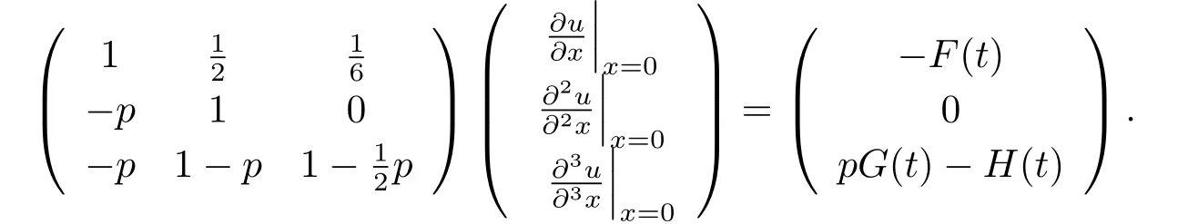
For the third type of boundary condition(III),by puttingx=1 into Eqs.(5.4)-(5.6)and using boundary conditions,we obtain a linear system ofwhich can be wri tten as
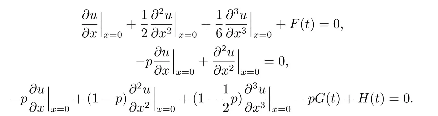
The matrix form of the above linear equations is given as follows
Solving this equations,we have
Therefore we have
and
Actually,the proposed method can be applied to solve the partial integro-differential equations with multiple weakly singular kernels.We consider the following problem

subject to the initial condition(1.2)and the second type boundary condition(II).We can handle the problem in previous way.Here we only derive the expression ofBy applying two times differentiation of (5.15) with respect tox,we get
Thus
6.Numerical Examples
In this section,we give some numerical examples for the fourth-order PIDEs with three types of boundary conditions to demonstrate the efficiency and reliability of the proposed method and the PIDE with two weakly singular kernels is also considered.
Example 1Consider the following partial integro-differential equation

subject to the initial condition

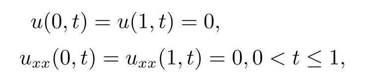
and the first type of boundary condition (I),

The exact solution of the problem is
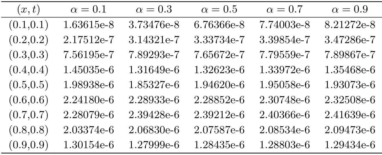
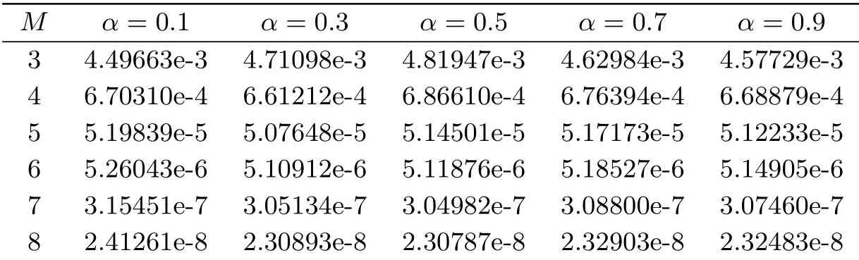
The problem is solved with different values ofα.Fig.1 shows the approximate solution and the absolute error of this problem in the case ofα=0.3,k=2 andM=6.Tab.1 lists the absolute error for different values ofαat different points withk=2,M=6.Tab.2 and Tab.3 give the maximum absolute error (L∞) obtained by the proposed method for different choices ofMandαat the points (xi,tj),wherexi=i/40,tj=j/40,i,j=0,1,2,···,40.
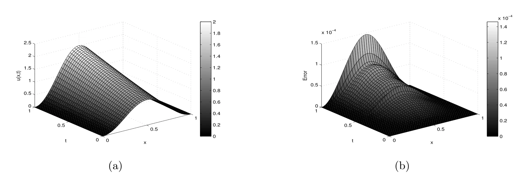
Fig.1 Approximate solution (a) and absolute error (b) for Example 1 with α=0.3, k=2 and M=6
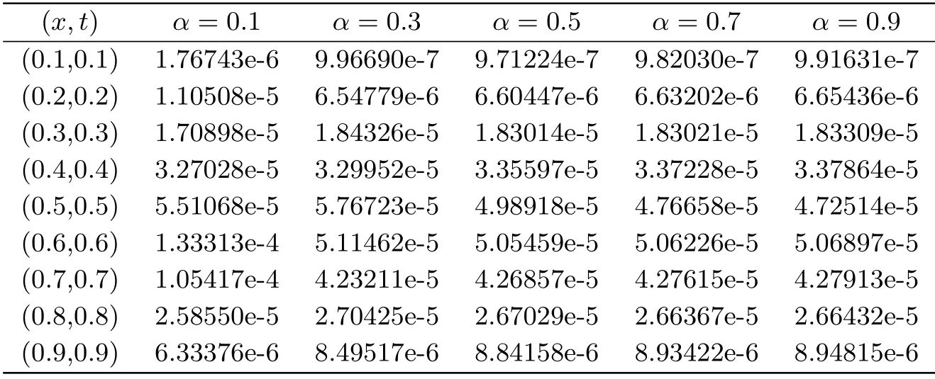
Tab.1 The absolute error of Example 1 for different α at some different points
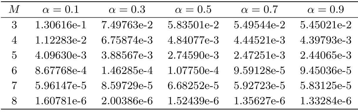
Tab.2 Maximum absolute error of Example 1 with various choices of M,α and k=2

Tab.3 Maximum absolute error of Example 1 with various choices of M,α and k=3
Example 2Consider the following partial integro-differential equation

subject to the initial condition

and the second type of boundary condition (II),
wheref(x,t)=(2t+1)sin(πx)+Γ(1−α)π4sinπx
The exact solution of the problem is

The problem is solved with different values ofα.Fig.2 plots the approximate solution and the absolute error of this problem in the case ofα=0.5,k=2 andM=6.Tab.4 shows the absolute error for different values ofαat different points withk=2,M=6.Tab.5 gives the maximum absolute error (L∞) obtained by the proposed method for different choices ofMandαat some points (xi,tj).

Fig.2 Approximate solution (c) and absolute error (d) of Example 2 with α=0.5, k=2 and M=6
Tab.4 The absolute error of Example 2 for some different α at some different points
Tab.5 Maximum absolute error of Example 2 with various choices of M and α
Example 3Consider the following partial integro-differential equation

subject to the initial condition

and the third type of boundary condition (III),
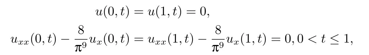
The exact solution of the problem is

The problem is solved with different values ofα.The graph of the approximate solution and the absolute error of this problem in the case ofα=0.7,k=2 andM=6 is shown is Fig.3.Tab.6 shows the absolute error for different values ofαat different points withk=2,M=6.Tab.7 gives the maximum absolute error(L∞)obtained by the proposed method for different choices ofMandαat some points (xi,tj).

Fig.3 Approximate solution (e) and absolute error (f) for Example 3 with α=0.7, k=2 and M=6

Tab.6 The absolute error of Example 3 for some different α at some different points
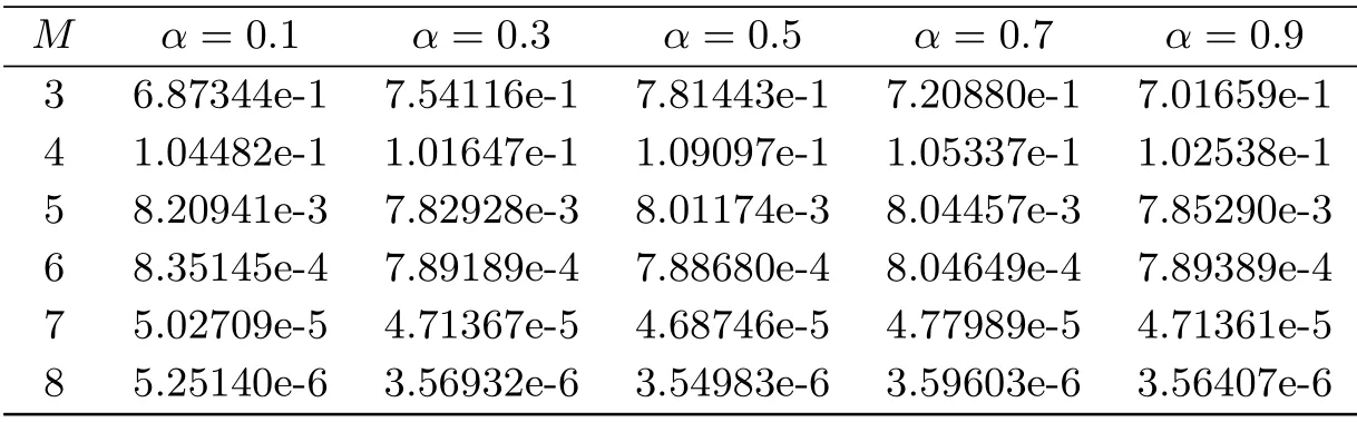
Tab.7 Maximum absolute error of Example 3 with various choices of M and α
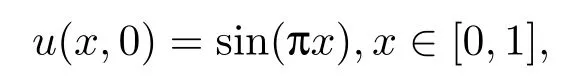
Example 4Consider the following partial integro-differential equation with two weakly singular kernels

subject to the initial condition
and the second type of boundary condition (II),

wheref(x,t)=(2t+1)sinπx+Γ(1−α)π2sinπx
The exact solution of the problem is

This problem is solved in the case of different values of (α,β).Fig.4 demonstrates the approximate solution and the absolute error of this problem in the case ofα=4/5,β=9/10,k=2 andM=6.Tab.8 shows the absolute error for different values of (α,β) at different points withk=2,M=6.Tab.9 gives the maximum absolute error (L∞) obtained by the proposed method for different choices ofMand (α,β) at some points.
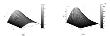
Fig.4 Approximate solution (g) and absolute error (h) for Example 4 with α=4/5,β=9/10, k=2 and M=6

Tab.7 The absolute error of Example 4 for different α and β at some points
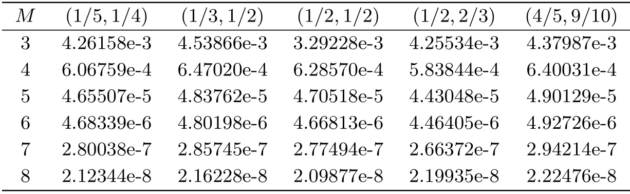
Tab.8 Maximum absolute error for Example 4 with various choices of (α,β) and M

Fig.5 Error as a function of the polynomial degree for various values of α and β
Remark 6.1Finally,we present the errors as a function of the polynomial degree for the all examples with different values ofαandβin Fig.5,where a logarithmic scale is used for the error axis.It is obviously that the errors appear in an exponential decay.Since one can obverse that the error variations are essentially linear versus the polynomial degrees in this semi-log axis.
7.Conclusion
In this paper,wavelet collocation method based on the fourth kind Chebyshev wavelets has been applied to a class of PIDEs with a weakly singular kernel.We derived the fractional integral formula of a single Chebyshev wavelet in the Riemann-Liouville sense via the shifted Chebyshev polynomials.The convergence analysis of two-dimensional fourth kind Chebyhev wavelets was studied.By applying fractional integral formula and fourth kind Chebyhev wavelets together with collocation method,PIDEs with a weakly singular kernel are reduced to a system of algebraic equation.The proposed method is very convenient for solving PIDEs,since the initial and boundary conditions are taken into account automatically when constructing the expression of the approximate solution to the problem.Several numerical examples are given to show the applicability and accuracy of the proposed method.