Multi-objective Optimization of a Fan Airfoil Adaptive for the Inlet Distortion*

Meng-yu Chen Ha-nan Lu Tian-yu Pan Qiu-shi Li

(1.National Key Laboratory of Science and Technology on Aero-Engine Aero-Thermodynamics,School of Energy and Power Engineering,Beihang University,Beijing,China；2.Collaborative Innovation Center of Advanced Aero-Engine,Beijing,China;3.Chengdu Aircraft Industrial(Group)Co.,Ltd.,Chengdu,China)

Abstract：Boundary Layer Ingestion(BLI)propulsion systems can significantly reduce the aircraft fuel burn but it can bring the inlet distortion problem to the fan and reduce its aerodynamic performance.To reduce the profile loss and enhance the distortion-tolerant ability of a fan airfoil operating under the fixed inlet distortion,this paper presents an optimization strategy for a controlled diffusion airfoil (CDA) optimization through the multi- objective genetic algorithm (MOGA) with Back-Propagation (BP) neural network.The optimization objectives are to minimize the profile loss and its sensitivity to the incidence angle.After the optimization,a fan airfoil adaptive for the fixed inlet distortion has been obtained.Compared with the conventional CDA,the profile loss of this fan airfoil is decreased under the positive incidence, and its sensitivity to the incidence angle is decreased by 32%. Simultaneously, the low loss incidence range is widened by 21%.

Keywords：Inlet Distortion,Fan Airfoil,Profile Loss,Multi-objective Optimization

Nomenclature

cchord length

MaMach number

βflow angle

Aamplitude of the distortion

wwidth of the distortion

p*total pressure

T*total temperature

Tperiod of the inlet distortion boundary

Cpstatic pressure coefficient=(p-p1)/(0.5ρ)

p static pressure

ωtotal pressure loss coefficient=/(0.5ρ)

σ(ω)standard deviation of the total pressure loss coefficient

V velocity

ρ objective

△βflow turning angle=β2-β1

i incidence angle=β1k-β1

Subscripts

0 undistorted region

1 inlet

2 outlet

minminimum

basebaseline

objobjective

1 Introduction

With the rapid development of the modern aircrafts,the fuel consumption has become important for the aircraft performance. Many previous system studies conducted by Geiselhart et al. (2003)[1], Plas (2006)[2], Nickol (2009)[3]have shown that the BLI propulsion systems can make an achievement of 5 to 10 percent reduction in aircraft fuel consumption. Since the BLI propulsion systems have significant potential for further fuel burn reduction, they have gained more and more attention.

For a BLI propulsion system, the fan would always operate under the severe inlet distortion due to the ingestion of the boundary layer from the aircraft surface.The inlet distortion would significantly deteriorate the aerodynamic performance of fan and further increase the aircraft fuel consumption. Therefore, it is very important to reduce the impacts of the inlet distortion on the fan performance.

Over the past decades, many efforts have been devoted to the investigations on the fan/compressor inlet distortion problem. Some researchers have developed theoretical prediction models to predict the flow instability of the fan/compressors under the inlet distortion condition. Pearson and McKenzie (1959)[4]developed a parallel compressor model for single distorted region. Subsequently, some improvement work based on the original parallel compressor model has been conducted by Adamczyk (1974) [5] and Mazzawy(1977)[6]. Hynes and Greitzer (1987)[7]developed a model to predict the onset of flow instability for an axial compressor under the circumferential inlet distortion.With respect to the influence of the inlet distortion on the flow losses in the fan/compressors,Hah et al.(1998)[8]numerically and experimentally studied the impacts of the inlet total pressure distortion on a transonic compressor rotor,and it was found that when the blade encountered the distorted region, the strong shock-boundary layer interaction would occur. Gunn and Hall (2014)[9] demonstrated that the inlet distortion would result in wide variations in the transonic fan rotor shock structure and strength, and the shock-boundary layer interaction would generate losses, thus decreasing 1 to 2 percent of the fan efficiency. Recently, Plourde and Stenning (2015)[10] demonstrated that the attenuation of the circumferential inlet distortion was mainly dependent on the slope of the pressure rising characteristic.

In the scope of the open literatures reporting the fan/compressor inlet distortion problem, there are still few reports concerning the design and optimization for the fan/compressors. Since the fan flow field under the inlet distortion is strongly unsteady and the three-dimensional (3D) unsteady calculation is very time-consuming, an investigation based on the two-dimensional (2D) airfoil is carried out in this paper. To obtain a fan airfoil adaptive for the inlet distortion, a 2D optimization strategy based on the inlet distortion condition is established in this paper. Under the inlet distortion condition, the airfoil inflow incidence would periodically change in a wide incidence range. Hence, the evaluation parameters of the airfoil performance under the inlet distortion should include not only the profile loss,but also its sensitivity to the variation of the incidence angle.

For the 2D blade airfoils, the CDA has been widely used due to its performance advantages.The previous experimental studies conducted by Hobbs and Weingold (1984)[11], Dunker et al. (1984)[12] have shown that the CDA has a wide range of stall-free incidence.This feature of the CDA make it better adapt to the variations of the incidence angle under the inlet distortion condition. Therefore, a conventional CDA is selected as the baseline airfoil for the present work.

In this paper, an integrated multi-objective optimization strategy has been developed for a CDA working under the fixed inlet distortion aiming at reducing both the profile loss and the performance sensitivity to the incidence angle. The Bezier curve is firstly used for airfoil parameterization and the sensitivity analysis is employed to select the design variables. Meanwhile, the sample database is established on the basis of the unsteady simulation method. Furthermore, the multi-objective optimization is carried out by using the MOGA coupled with BP neural network to obtain the optimal design.

2 Numerical Simulation Method

2.1 Baseline Airfoil

In this paper, a conventional CDA is used as the baseline airfoil.The CDA has been widely used as the baseline in the turbomachinery design and optimization (Obayashi et al.(2000)[13], Sonoda et al. (2003)[14]). Table 1 summarizes the design parameters and conditions of this CDA.

Tab.1 Design parameters and conditions of the CDA

2.2 Numerical Method

The airfoil aerodynamic performance is obtained by solving the 2D unsteady compressible Reynolds-averaged Navier-Stokes equations using the ANSYS FLUENT through a finite volume method. The continuity, momentum and energy equations are solved through the pressure-based coupled algorithm. The advection term is discretized by the second-order upwind scheme, and the diffusion term is discretized by the second-order central-differencing scheme.The implicit time integration scheme is employed by setting the physical time step and the maximum internal time step to be 10-5and 25, respectively. The k-ε model is used as the turbulence model.

The computational mesh is generated using the ICEM.The whole computational domain considers 20 airfoil passages to simulate the real scale of the inlet distortion condition.Figure 1 shows the schematic of the two adjacent passages in the computational domain. The lengths of the upstream and downstream of the airfoil passages are both set to be 1.5D(D=20t/π), so that the inlet and outlet boundaries will not be affected by the perturbations of the flow around the airfoils.Additionally,the structured grid is used for the entire computational domain, and the near wall grid is adjusted to keep y+≤5. Furthermore, a relative coordinate system translating in the negative direction of the y-axis is imposed on the entire computational domain.

A grid-independence study is implemented to eliminate the impact of the grid size on the numerical results. The calculations are conducted with three different mesh sizes by imposing the same inlet and outlet conditions on the computational domain. As shown in Figure 2, the obtained total pressure loss coefficient and the flow turning angle change slightly from Grid B to Grid C.Thus,considering the computational time and accuracy, the total number of grid nodes is set to be approximately 0.3 million (Grid B) in this present work.

For the unsteady simulations, the residual values of the velocity components and the pressure are all specified to be less than 10-4for the convergence. The method for determining convergence is to monitor the pressure ratio to fluctuate periodically; meanwhile, the variations of the pressure ratio at the corresponding time of two adjacent periods should be less than 5%.

2.3 Validation of Numerical Method

Since there is no experimental data available considering the inlet distortion working condition,the flow field cannot be directly compared between the experimental and numerical data. Therefore, a computational fluid dynamics(CFD) validation is conducted based on the experimental data under the clean inflow condition obtained by Elazar and Shreeve(1990)[15].Figure 3 shows the numerical and experimental results of the static pressure coefficient distributions on the CDA surface at the design point.As can be seen from this comparison, the CFD results agree well with the experimental data.The result indicates that the CFD tool and method adopted in this work are reliable and can be used to predict the flow field in the present work.

2.4 Inlet Total Pressure Distortion Condition

The inlet distortion boundary condition has been obtained through the following analysis. For a given inlet distortion distribution, the flow parameters at any point on the inlet boundary in the absolute coordinate system is a function of both time and space which can be expressed as follows:

where q represents the flow physical parameter, e.g. total pressure and total temperature. The r, θ and z represent the absolute coordinates.For a stable distortion,the q can be simplified into a space function of θ with a period of 2π.

Assuming that the rotational speed of a compressor rotor is Ω and the time in relative coordinate is t.Thus,the relation of the distortion distribution in the relative and absolute coordinates can be expressed as follows:

Therefore, the flow parameter at a point on the inlet boundary in the relative coordinate will be

where f(t) denotes the time-domain function of the flow parameters in the relative coordinate.

Based on the above analysis, the space-domain function of the flow parameters can be changed into the time-domain function. In this work, the inlet distortion condition is simplified into a cosine form function based on the mid-section(marked with dash line in Figure 4)of the BLI inlet total pressure distribution obtained by Florea et al. (2015)[16].The mathematical expression of the unsteady total pressure distortion can be defined as follows:

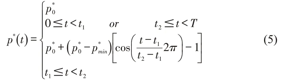
Fig.1 Schematic of the computational mesh

Fig.2 Grid-independence study

Fig.3 Comparison of static pressure coefficient distributions

Fig.4 BLI inlet total pressure distribution

At the inlet, the total pressure and total temperature are specified along with the flow angle. At the outlet, the average static pressure is specified.The unsteady inlet total pressure condition is embedded into the FLUENT code through the User Defined Function(UDF).As shown in Figure 5,the cosine form total pressure distortion translates periodically at the inlet boundary.To study conveniently,two parameters describing the intensity of the distortion are defined, one is the amplitude of the distortion A, and the other is the width of the distortion w. Specific parameters of the inlet boundary are set as follows:

It is worth mentioning that the relative motion between the inlet boundary and the airfoils only results from the motion of the inlet distortion condition, while the airfoils remain stationary. In addition, the relative coordinate system is only employed to create the non-uniform incidence angles for the airfoils.

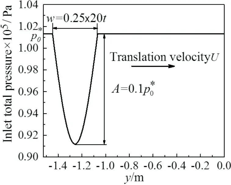
Fig.5 Schematic of the inlet distortion condition

3 Optimization Methodology

3.1 Airfoil Parameterization

To keep the curvature of the airfoil profile continuous and smooth, the Bezier curve based on the Bernstein basis function is used to parameterize the airfoil. A general n-parameters Bezier curve can be expressed as follows:

where pirepresents the x or y-coordinate of the control points and B(t) denotes the Bernstein basis function.The Bernstein basis function can be expressed as:

In the present work,the airfoils are generated by imposing the thickness on the mean camber line. As depicted in Figure 6, considering the fitting accuracy and optimization efficiency, the mean camber line and thickness distributions are fitted by the fifth and seventh order Bezier curves,respectively.

To parameterize the suction surface (SS) and pressure surface (PS) of the baseline airfoil, a total number of 200 control points are used. Figure 7 shows a comparison between the parameterized airfoil and the baseline airfoil. It can be seen that the parameterized airfoil agree well with the baseline airfoil.

Fig.6 Results of the airfoil parameterization

Fig.7 Comparison of the baseline airfoil points and parameterized airfoil

3.2 Optimization Strategy

To conduct the optimization, an integrated optimization strategy is developed. The optimization strategy consists of four key components: an airfoil parameterization technique,an efficient design of experiment (DOE) method, a reliable flow solver,and an optimization toolkit.A detailed optimization process is shown in Figure 8.

The optimization process starts with the airfoil parameterization.Simultaneously,the optimization objectives are determined and the design variables are selected through sensitivity analysis. Then, the Latin Hypercube Sampling (LHS)is used to establish a sample database through a limited number of sample points whose aerodynamic performance can be predicted by the numerical simulations.The sample database is used to develop a surrogate model to predict the aerodynamic performance of the investigated airfoil. In this paper,the BP neural network is employed as the surrogate model.Finally, the MOGA is adopted to obtain the Pareto optimal solutions. In this work, the operation parameters of the MOGA are set as follows: the population size is 50, the number of generation is 100, the crossover probability is 0.9 and the mutation probability is 0.01.

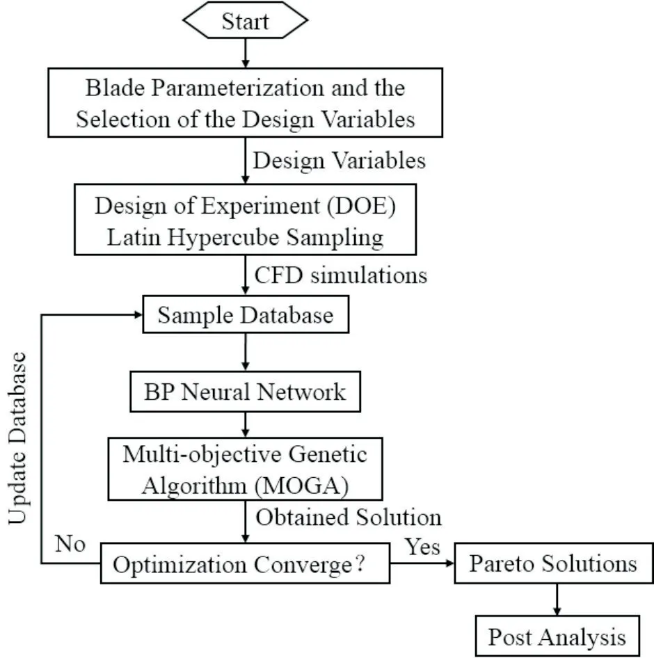
Fig.8 Flow chart of the optimization process

3.3 Optimization Design Problem Description

An optimization problem can be described by three basic elements: the optimization objectives, design variables and constraints.These three basic elements will be described in the following parts.

3.3.1 Objectives

When an airfoil operates under the inlet total pressure distortion,the airfoil inflow incidence angle will change periodically in the positive incidence range. Therefore, the optimization objectives should be set for two aspects. One is to reduce the profile loss under the positive incidence working conditions, and the other is to reduce the sensitivity of the loss to the variation of the positive incidence.

As shown in Figure 9, it is possible to reduce the profile loss in the positive incidence range by reducing the loss at the incidence angle operating point OPT2. Meanwhile,the sensitivity of the loss to the positive incidence can be reduced by decreasing the slope of the right branch of the loss-incidence characteristic.These two objectives can be expressed as Equations(8)and(9),respectively.

The total pressure loss coefficient has been widely used to evaluate the loss in the turbomachinery design. The total pressure loss coefficient in the compressible flow can be defined as follows:

In this paper, the standard deviation of the total pressure loss coefficients at four incidence angles (marked with red circles in Figure 9) is employed to evaluate the sensitivity of the profile loss to the positive incidence. The specific definition can be written as:

where n=4, ωirepresents the total pressure loss coefficient at the i th incidence angle, and-ω is the average value of the total pressure loss coefficients at the four incidence angles.

3.3.2 Design variables

In this work, the airfoil thickness distribution is kept constant during the whole optimization process,and the coordinates of the control point P1to P4on the mean camber line in Figure 6(a)are used to change the shape of the airfoil.

Since different variables would have different impacts on the two objective functions ( ωOPT2and σ(ω)), the influence of each variable on the objective functions is investigated through sensitivity analysis. The sensitivity tests are conducted by changing the value of each variable while keeping the remaining variables fixed. The variables having significant influences on both objective functions are selected as the design variables.

Fig.9 Demonstration of the operating points

Figure 10 shows the results of the sensitivity tests for the main variables, where the x or y in the horizontal coordinate subscript represents the x or y coordinate of a control point. To study conveniently, the values of the ωOPT2and σ(ω) are correspondingly normalized by those of the baseline airfoil. It can be seen from Figure 10:①The two objectives( ωOPT2and σ(ω))are more sensitive to the movements of the control points P1and P2near the LE. However, the movements of the control points P3and P4near the TE have slight influences on the two objectives;②As the x and y coordinates of the control points increase, the P1is decreased first and then increased,and the σ(ω)is gradually decreased.

Further, to quantify the influence of the each variable on the two objectives ( σ(ω)and σ(ω)), Figure 11 shows the proportion of the influence of each variable on the two objectives. The results show a similar trend as depicted in Figure 10 and indicate that the variations of the control points P1and P2have greater impacts on the two objectives than those of the control points P3and P4.To reduce the design space, only four variables accounting for more than 10% of the proportion of the influence are selected as the design variables, namely, the x and y coordinates of the control points P1and P2. Meanwhile, the design space can be determined according to the ranges of the four design variables.

Fig.10 Results of sensitivity analysis

Fig.11 Proportions of the influence of the main variables on the two objective functions

3.3.3 Constraints

The optimization is subject to the following constraints.

1. Geometrical constraint: to keep the airfoil thickness distribution and other geometrical parameters (e.g. stagger angle and solidity)constant.

2.Performance constraint:to keep the relative variation of the flow turning angles within 4%at OPT2.

where Δβobjand Δβbaserepresent the flow turning angles of the optimized and baseline airfoils.

3.3.4 Mathematical model

Based on the aforementioned descriptions of the present optimization problem, the mathematical model of the multi-objective optimization problem can be expressed as follows:

where x represents the design variable and the variation range of each variable is normalized.

4 Results and Discussion

4.1 Optimization Results

Figure 12 presents the multi-objective optimization results for the CDA under the inlet total pressure distortion.The values of ωOPT2and σ(ω)are correspondingly normalized by those of the baseline airfoil. Three optimization results(Design1,Design2 and Design3)are selected for further analyses. To be specific, the Design1 represents the result with the smallest σ(ω), the Design3 represents the result with the smallest ωOPT2, and the Design2 represents the result with both relative small σ(ω)and ωOPT2.

Figure 13 shows the comparison of the profiles between the baseline airfoil and the optimized airfoils. As can be seen from this figure, compared with the baseline airfoil,the curvatures of the optimized airfoils are all increased before the 40% chordwise location; however, after the 40% chordwise location, the profiles of the baseline airfoil and the optimized airfoils almost overlap.Here,the maximum deflections(divided by chord length)of the baseline airfoil,Design1,Design2 and Design3 are 0.32,0.36,0.35 and 0.33,respectively. Meanwhile, the maximum deflection positions(divided by chord length) are 0.55, 0.49, 0.50 and 0.52, respectively.

Fig.12 Multi-objective optimization results

Fig.13 Comparisons of the airfoils

Figure 14 compares the time-averaged loss-incidence characteristics before and after the optimization under the inlet distortion. The low loss incidence range Δi is introduced based on the report by KÖller et al. (1999)[17]. This range represents the incidence range when ω≤2ωmin. Since the airfoil would stall before operating at the incidence angle when ω=2ωmin, the Δi obtained in this work is calculated by extending the loss-incidence characteristic curve along the trend.It can be seen from this figure that:①The sensitivities of the profile loss to the incidence angle of the three optimized airfoils are all reduced;②The low loss incidence ranges of the three optimized airfoils are all widened; ③Above an incidence angle of 1°, the profile losses of the three optimized airfoils are all lower than those of the baseline airfoil.

Table 2 summarizes the time-averaged aerodynamic performance of the baseline airfoil and the optimized airfoils under the inlet distortion.Compared with the baseline airfoil,four conclusions can be drawn as follows:①As for Design1,the ωOPT2is increased by 1%, σ(ω)is decreased by 41%, and Δi is widened by 24%; ②As for Design2, the ωOPT2and σ(ω)are decreased by 0.2% and 32%, respectively. Meanwhile,the Δi is widened by 21%; ③As for Design3, the ωOPT2and σ(ω) are decreased by 2% and 23%, respectively. Meanwhile,the Δi is widened by 15%;④The flow turning angles of the three optimized airfoils at OPT2 (in Figure 9) are all slightly increased, but the increments are all within the constraint range.

Fig.14 Comparisons of time-averaged loss-incidence characteristics under the inlet distortion

Tab.2 Comparisons of time-averaged aerodynamic performance under inlet distortion

Based on the trade-off analysis, the Design2 can best meet the two objectives for both reducing the profile loss over the whole positive incidence range and decreasing the sensitivity of the loss to the incidence angle. Therefore, the Design2 is selected as the final optimization result in this paper.

4.2 Unsteady Analysis

To explore the physical mechanisms of the optimization results,the unsteady flow field analyses are given in this part.Since the design incidence of the baseline airfoil is 4.5°,and the total pressure distortion can lead the airfoil inflow incidence angle to periodically change in a wide positive incidence range, the flow field analyses are performed at OPT3(in Figure 9).

To conveniently analyze, one period of the total pressure distortion movement is divided into 20 moments and one moment means every time the total pressure distorted region passes a passage. Figure 15 shows the unsteady change of the airfoil inflow incidence angle during one period. As can be seen from the figure, the main incidence angles are positive during an unsteady period.Moreover,before the airfoil enters the distorted region,the incidence angle would decrease to a minimum value.After the airfoil entered the distorted region,the incidence angle would rapidly increase to a peak value, and then the incidence angle would be gradually back to normal after the airfoil left the distorted region.

To compare the profile loss between the baseline airfoil and the Design2,Figure 16 shows the comparisons of the entropy at four key moments of an unsteady period. The four moments in this figure correspond to the four moments marked in Figure 15. It is found that the development of the boundary layer is a dynamic process.At the moment t=0,the airfoils are in the undistorted region and the incidence angles are small.At this moment,the PS boundary layers of the Design2 are thicker, thus producing higher friction loss in the boundary layer. when t=(12/20)T, the airfoils are just entering the distorted region, the incidence angles remain relative small. At this moment, the comparisons of the profile loss are similar to those when t=0. When t=(14/20)T, the airfoils are moving into the distorted region and the incidence angles become relative large. At this moment, the LE separation bubbles on the SSs of the Design2 are smaller, which means the separation loss of the Design2 is lower. When t=(16/20)T, the airfoil LEs have partly left the distorted region, the high-energy fluid has flowed into part of the airfoil passages and promoted the low-energy fluid on the SSs to migrate and diffuse into the downstream. when, the separation loss of the Design2 is lower.

Further analyses indicate that the inlet total pressure distortion can make the incidence angle of the airfoil change periodically.When the incidence angle is relative large,the fluid would rapidly accelerate to the velocity peak at the SS front part due to the increase of the curvature of the SS front part of the Design2. In this situation, the length of the fluid deceleration region on the SS would be longer. It would be beneficial for reducing the separation loss in the boundary layer. When the incidence angle is relative small (in undistorted region or just entering the distorted region), due to the increase of the curvature of the PS front part of the Design2,the adverse pressure gradient on the PS would be larger, so that the PS boundary layer would be thicker, thus increasing the friction loss.

Fig.15 Unsteady change of the incidence angle

Fig.16 Comparisons of the entropy contours at OPT3

In spite of the higher friction loss at the relative small incidence angles, the separation loss of the Design2 is much lower than that of the baseline airfoil at the relative large incidence angles. Therefore, the overall profile loss of the Design2 is much lower than that of the baseline airfoil at OPT3.

5 Conclusions

In this paper, an integrated multi-objective optimization strategy for obtaining a fan airfoil adaptive for the fixed inlet distortion is developed. The proposed optimization strategy is applied to the optimization design of a CDA to achieve the lower profile loss in the positive incidence range and the lower sensitivity of the profile loss to the incidence angle. The multi-objective optimization is conducted by using the MOGA coupled with BP neural network. The following conclusions can be drawn:

1) Based on the sensitivity analysis, the two objectives are more sensitive to the movements of the control points near the LE than those of the control points near the TE.Furthermore, with the increase of the coordinates of the control point, the profile loss is decreased first and then increased,and its sensitivity to the incidence angle is decreased.

2)A fan airfoil adaptive for the inlet distortion has been obtained. From the LE to the 40% chord wise location, the curvature of the optimized airfoil is increased compared with that of the conventional airfoil and the maximum deflection position also moves forward. In the meanwhile, the profile loss of the optimized airfoil is reduced in the positive incidence range,and the sensitivity of the profile loss to the incidence angle is decreased by 32%. Simultaneously, the low loss incidence range is widened by 21%. Overall, the optimized airfoil has achieved the two objectives for both reducing the profile loss and improving the airfoil distortion-tolerant ability.

3) The fluid would rapidly accelerate to the velocity peak at the SS front part due to the increase of the curvature of the optimized airfoil front part.In this situation,the length of the fluid deceleration region on the SS would be longer.It would be beneficial for reducing the separation loss in the positive incidence range.