An integrated method of selecting environmental covariates for predictive soil depth mapping
2019-02-14LUYuanyuanLIUFengZHAOYuguoSONGXiaodongZHANGGanlin
LU Yuan-yuan , LIU Feng ZHAO Yu-guo , SONG Xiao-dong ZHANG Gan-lin
1 State Key Laboratory of Soil and Sustainable Agriculture, Institute of Soil Science, Chinese Academy of Sciences, Nanjing 210008, P.R.China
2 University of Chinese Academy of Sciences, Beijing 100049, P.R.China
Abstract Environmental covariates are the basis of predictive soil mapping. Their selection determines the performance of soil mapping to a great extent, especially in cases where the number of soil samples is limited but soil spatial heterogeneity is high. In this study, we proposed an integrated method to select environmental covariates for predictive soil depth mapping.First, candidate variables that may in fluence the development of soil depth were selected based on pedogenetic knowledge.Second, three conventional methods (Pearson correlation analysis (PsCA), generalized additive models (GAMs), and Random Forest (RF)) were used to generate optimal combinations of environmental covariates. Finally, three optimal combinations were integrated to produce a final combination based on the importance and occurrence frequency of each environmental covariate. We tested this method for soil depth mapping in the upper reaches of the Heihe River Basin in Northwest China. A total of 129 soil sampling sites were collected using a representative sampling strategy, and RF and support vector machine (SVM) models were used to map soil depth. The results showed that compared to the set of environmental covariates selected by the three conventional selection methods, the set of environmental covariates selected by the proposed method achieved higher mapping accuracy. The combination from the proposed method obtained a root mean square error (RMSE) of 11.88 cm, which was 2.25–7.64 cm lower than the other methods, and an R2 value of 0.76,which was 0.08–0.26 higher than the other methods. The results suggest that our method can be used as an alternative to the conventional methods for soil depth mapping and may also be effective for mapping other soil properties.
Keywords: environmental covariate selection, integrated method, predictive soil mapping, soil depth
1. Introduction
Soil mapping, classification, and pedologic modeling have been important drivers in the advancement of our understanding of soil from the earliest scientific studies of soils (Breviket al.2016). Digital (or predictive) soil mapping methods provide a rapid and inexpensive way to predict soil types or properties over large areas (Scullet al.2003;Yanget al. 2015; Minasny and McBratney 2016; Pásztoret al.2016; Zhanget al.2017). Soil-landscape models that characterize soils as a function of environmental variables, including climate, organisms, topography, parent material, and time, are the theoretical basis for predictive soil mapping. Specific landscape factors determine the formation of specific soil properties. The spatial distribution patterns of soil types or properties result from the interactive action of multiple soil-forming factors (Jenny 1994; Hudson 1992; McBratneyet al.2003). With the rapid development of geographical information techniques and remote sensing products, numerous datasets of environmental variables have been acquired. These variables can characterize soil-forming factors from multiple aspects. However, a problem also arises: how to select an optimal combination of environmental variables to achieve accurate and steady soil mapping performance? This is an important issue in digital soil mapping because not all environmental covariates have equal predictive capability in modeling, and some covariates may cause noise that reduces the predictive capability of the employed models (Buiet al.2016). Variable selection attempts to identify and remove the variables that penalize the performance of a model because they are useless,noisy, redundant, or correlated by chance (Zouet al.2010;Liuet al.2016). Liuet al.(2009, 2012) discussed the issue of environmental covariates in low relief areas. Behrenset al.(2010) observed that the selection of features appears to aid in the interpretation of data about soil formation and that only a small number of features are typically required to achieve good predictions. Variable selection aims to work with fewer covariates and thus simplify the predictive model,allowing for better computing ef ficiency without decreasing the performance of model (Lacosteet al.2016). Variable selection can also provide robust models that may be readily transferred, and it allows non-expert users to build reliable models with only limited expert intervention (Zouet al.2010).
Pearson correlation analysis (PsCA) is the most common method for variable selection. As commonly used modeling methods, generalized additive models (GAMs)and Random Forest (RF) algorithms not only can select variables in their own ways but can also be used for digital soil mapping. Rodriguez-Galianoet al.(2014) applied PsCA in combination with multiple linear regression to identify variables that were significantly correlated with soil organic matter. Tesfaet al.(2009), Zhiet al.(2017), and Heunget al.(2014) selected environmental variables that affected soil development based on variable importance determined by RF. Tesfaet al.(2008) and Denget al.(2015) extracted optimal environmental variables using GAMs. These studies demonstrated that the removal of non-informative variables can produce better prediction and simpler models.However, the three variable selection methods described above quantify the predictive capability of environmental variables based on different mechanisms. Each method has its strengths and weaknesses, and no studies to date have determined which method is the best suited to a particular data, so it is dif ficult to choose an optimal method of variable selection. In addition, the digital soil mapping performances of the corresponding optimal combinations selected by the different methods are not steady. The performance of a combination is often related to its original selection method.For example, for an optimal combination selected by GAMs,the prediction result of GAMs usually outperforms other methods (such as RF), andvice versa. Therefore, there is still a need to explore a new variable selection method for digital soil mapping studies.
We choose soil depth as the target soil property for studying environmental variable selection and digital soil mapping. One reason for investigating soil depth is that it is an important input parameter for hydrological and ecological modeling. It can affect hydrological processes(Lianget al.1996; Schenk and Jackson 2005; Tesfaet al.2009), in fluence soil quality and productivity (Poweret al.1981), determine the soil’s capacity to store and hold moisture (Boeret al.1996), and control the soil’s surface and subsurface processes (Heimsathet al.2001). Soil depth is also a necessary parameter when calculating carbon and other elemental stocks. Additionally, it is often dif ficult to accurately map soil depth due to its high heterogeneity and dif ficulty of data collection, especially in mountainous areas. Being able to predict the soil depth in the complex landscape areas can lead to a better understanding of soil erosion or water storage (Hudson 1992; Dietrichet al.1995;Luet al.2014; Scarponeet al.2016).
The objective of this study is to propose a new method of selecting environmental covariates, test its effectiveness through the use of the selected covariates for predictive soil depth mapping and compare it with current variable selection methods.
2. Materials and methods
2.1. Study area
The study area covered approximately 30 000 km2in the upper reaches of the Heihe River Basin in Northwest China, on the northeast margin of the Tibetan Plateau(latitude 37.71° to 40.03°N, longitude 96.78° to 101.2°E)(Fig. 1). This region is dominated by the Qilian Mountains,which range in elevation from 1 684 to 4 600 m above sea level with an average of 3 535 m. The study area has a typical plateau continental climate, and the mean annual temperature ranges from –12.3 to 6.6°C. The mean annual precipitation ranges from 480 mm in the southeast to 80 mm in the northwest, with a mean value of 300 mm.
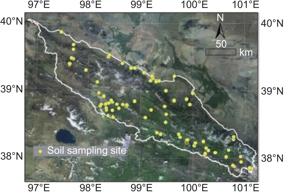
Fig. 1 Location of study area and soil sampling site.
As a result of the special hydrothermal conditions and the undulating relief, the region has a notable vertical zonal vegetation pattern (Wanget al.2016). There are a rich variety of soil types in this study area, mainly including Inceptisols, Gelisols, Entisols, Aridisols, and Histosols,according to Soil Taxonomy (SSS 2010). In addition, the parent materials are complex and diverse, mainly including moraine deposits, slope deposits, residual deposits, alluvialdiluvial deposits, gully deposits, alluvial deposits, etc. (Li Xet al.2017). Due to the complex topographical conditions,various types of landforms are dominated by high and medium-height mountains, hills, plains, platforms, river terraces, and floodplains, which were formed by various processes, such as glaciation, periglaciation, and erosion.
2.2. Soil sampling
Soil surveys were conducted during July and August of 2012 and 2013, and 129 soil pro files were studied (Fig. 1).Due to the low accessibility of the alpine environment, a purposive sampling strategy (Zhuet al.2008) was adopted to determine representative sampling sites. During the sampling process, detailed information about the locations of the sampling sites, including the characteristics of the landscape environment, vegetation, and rock distribution,was recorded. In addition, the soil pro file at each sampling site was described in several pedogenetic horizons based on main morphology of horizons. Based on the above information, the soil depth at the sampling site was determined. In this study, soil depth refers to the solum thickness, which is the distance from the surface to the upper boundary of the “non-soil mass”, which is either bed rock or material that contains >75% by volume of>2 mm gravel. For more details, readers can refer to Yiet al.(2015).
2.3. Environmental variables
In this study, the following environmental variables were selected to set up and test the selection methods.
A digital elevation model (DEM) and its derivativesA freely available DEM was acquired from a Shuttle Radar Topography Mission DEM (SRTM DEM) with a resolution of 90 m. Seven topographic attributes, including elevation(ELE), slope, aspect, plan curvature (Plancur), pro file curvature (Procur), topographic wetness index (TWI), and vertical distance to channel network (VDCN), were derived from the DEM using the System for Automated Geoscientific Analyses (SAGA) geographic information system. Three types of transformation were employed for the aspect. The original aspect had a value between 0 and 360°. The first transformation was expressed in absolute values between 0 and 180°, which represented north and south, respectively,and was denoted by deviN. The second transformation, in which a cosine transformation was applied to converting the aspect into a range from 0 to 1, was denoted by cos_Asp.The third was the cosine transformation of deviN, which was denoted by cos_dN.
Climate dataMean annual temperature (MAT), mean annual precipitation (MAP), and drought index (DI) during the previous 30 years were derived as 1-km grids from the interpolation of data from 673 meteorological stations in China.
Landsat 5 Thematic Mapper (TM) imageryCompared to the other remotely sensed images, the Landsat 5 TM image was chosen to represent the “organism” soil-forming factor in this study by its ability of multichannel observation with a frequent revisiting period, fine high spatial resolutions, and free availability. A 30 m Landsat 5 TM mosaic image was acquired from the Cold and Arid Regions Sciences Data Center in China (DCHP 2011). The visible-red band (B3,0.63–0.69 μm), near-infrared band 4 (B4, 0.76–0.96 μm)and shortwave infrared band 5 (B5, 1.55–1.75 μm) were retained. To represent the vegetation intensity, we used the normalized difference vegetation index (NDVI), which was calculated as (B4–B3)/(B4+B3).
To take advantage of relatively detailed terrain information,the environmental variables were collected and converted into raster format with a 90-m resolution using ArcGIS 9.3(ESRI Inc., USA). The spatial distributions of the main environmental variables are presented in Fig. 2.
2.4. An integrated method for covariate selection
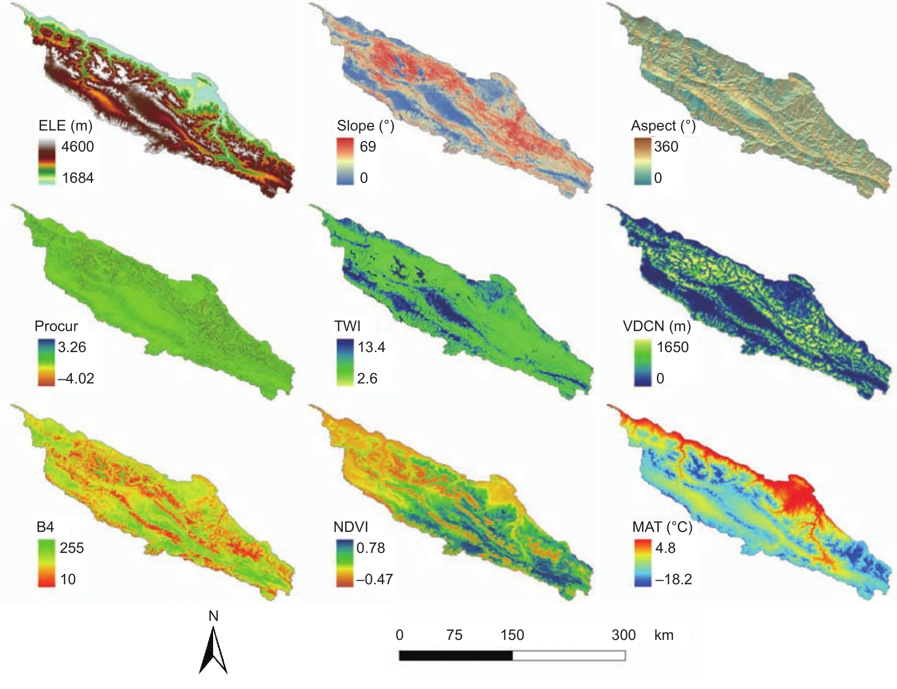
Fig. 2 Spatial distributions of environmental variables in this study area. ELE, elevation; Procur, pro file curvature; TWI, topographic wetness index; VDCN, vertical distance to channel network; B4, Landsat 5 TM band 4; NDVI, normalized difference vegetation index; MAT, mean annual temperature.
The integrated method (IM) consisted of three main steps(Fig. 3). First, we applied pedogenetic knowledge in the area of interest to determine candidate environmental variables for soil depth prediction. Second, three conventional variable selection methods (PsCA, GAMs and RF) were used to derive three optimal combinations of environmental variables, namely, PsCA_v, GAMs_v, and RF_v, respectively. Third, a comprehensive process was conducted on the three optimal variable combinations to generate a set of comprehensive covariates, which was denoted by IM_v.
Selection of candidate covariates based on pedogenetic knowledgeThe genesis and development of soil depth are the result of the interactive action of topographical, climatic,biological, and other factors. Therefore, selecting the environmental variables affecting soil depth development is the key to digital soil mapping. Pedogenetic knowledge and previous research on the soil depth indicate that topography is an important factor that affects soil formation and development, particularly in alpine areas (Gessleret al.1995; Böhner and Selige 2006; Körner 2007; Buolet al.2011; Sarkaret al.2013). Topography in fluences soil development by affecting the redistribution of watertemperature conditions and soil matter. In mountainous areas, soil at the tops of slopes generally moves outward and downward due to the effects of flowing water and gravity,and it ultimately deposits in valleys or lower and more gently sloped areas. Hence, many factors, including elevation,slope gradient and orientation, surface roughness, water distribution, and distance from watercourses, may affect the transport distance and velocity as well as the deposition location. Moreover, temperature and precipitation vary with elevation in alpine areas; therefore, the vegetation varies with elevation and climatic factors. The interaction of a multitude of factors comprehensively affects the development of soil depth.
This study analyzes the relationship between soil depth and the soil-forming environment. Environmental variables that affected the genesis and development of soil depth were selected based on pedogenetic knowledge and are referred to as candidate variables. This method of selecting candidate variables is called the pedogenetic knowledge(PG) method. The combination of candidate variables is denoted by cand_v. A total of 17 variables, elevation,slope, aspect, cos_Asp, deviN, cos_dN, Plancur, Procur,TWI, VDCN, MAP, MAT, DI, B3, B4, B5, and NDVI, were selected for cand_v.
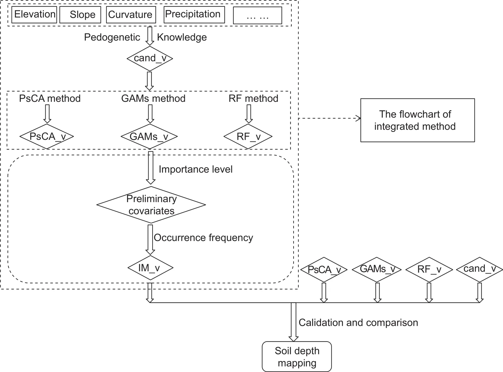
Fig. 3 Flowchart diagram of this study. PsCA, GAMs, RF represent the covariate selection methods of Pearson correlation analysis, generalized additive models and Random Forest; cand_v, PsCA_v, GAMs_v, RF_v, IM_v represent the combinations of environmental covariates derived from pedogenetic knowledge, PsCA, GAMs, RF and the integrated method.
Derivation of multiple optimal covariate combinationsfrom different selection algorithmsPsCA, GAMs and RFs methods were used to select optimal combinations of covariates. The basic principle and selection processes of the three methods are as follows:
(1) Pearson correlation analysis (PsCA)
The Pearson correlation coef ficient can be used to determine the degree of linear correlation between two series and is obtained by dividing the standard deviations of two variables by their covariance. The calculation function is defined as following (Tang 2008):
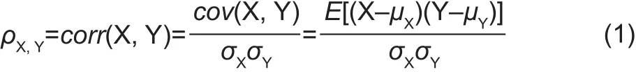
Where,ρX,Yis the Pearson correlation coef ficient;XandYare two variables;cov(X,Y) is the covariance betweenXandY;σXandσYare the standard deviations ofXandY, respectively;μXandμYare the means ofXandY,respectively; and E is the expectation.
The PsCA can be used to calculate the correlation coef ficient andP-value between the predictor and response variables or among the predictor variables. First, the variables significantly correlated with soil depth at a statistical level of 0.05 were selected. Subsequently, the multicollinearity among variables was checked, and the variables with the lowest correlation coef ficient were removed. Finally, the environmental variables were gradually selected to form an optimal combination of environmental covariates (denoted by PsCA_v). The PsCA method was implemented using the “psych” package in the Statistical Software R 3.1.2(R Development Core Team 2014).
(2) Generalized additive models (GAMs)
GAMs, which was proposed and developed by Hasitie and Tibshirani (1990), is non-parametric extensions of generalized linear models. The advantages of GAMs are that they are capable of directly dealing with the nonlinear relationships, identifying the data structure and determining the data pattern using non-parametric methods, and “talking”using data instead of models, and they do not require an assumed data distribution. In addition, GAMs are capable of examining the importance of each factor and selecting the optimal model. The expression is as follows:

Where,g() is expressed as a sum of the link functions of each variable;μis the expectation of the response variable;αis the intercept or constant term;mis the number of independent variables; andfjis an unspeci fied smoothing function, which can be obtained by a smoothing method,such as a locally weighted regression or spline function.
The spline smooth function is applied in this study.
Based on the combinations of cand_v, the single-factor analysis and multi-factor analysis were performed to select the environmental factors that played dominant roles in the model. According to the size and level of the estimated degrees of freedom and concavity, the optimal combination of environmental factors was obtained based on the GAMs method (denoted by GAMs_v). The GAMs method was implemented using the “mgcv” Package in R (Wood 2001).
(3) Random Forest (RF)
RF is a powerful ensemble-learning algorithm based on the classification and regression tree (Breiman 2001).The principle of RF is to grow several tree models using random samples and random feature selection techniques and then aggregate these tree models into a comprehensive classi fier. During the generation process of RF, each tree is grown using approximately two-thirds of the training data,and the other third is used as out-of-bag (OOB) error data for validation. In this study, we adopted the mean decrease in accuracy (MDA) as the variable importance index. For the regression, the MDA was the average increase in the squared OOB residuals when the variable was permuted(Liaw and Wiener 2002).
The optimal covariates were selected based on the variable importance calculation by RF. In other words,a model was first established based on the candidate variables, and the variables were then sorted based on their importance. Subsequently, the variable with the lowest importance was eliminated. This process was repeated until an optimal combination of covariates (denoted by RF_v)was selected. During this process, the relative importance of each environmental variable was evaluated based on the average of 100 repetitive calculations. The “randomForest”package in R was used to establish the relationships between soil depth and predictor variables.
Generation of final covariate combination through a comprehensive processThe three optimal combinations of environmental covariates (i.e., PsCA_v, GAMs_v, and RF_v) were obtained using conventional selection methods(PsCA, GAMs, and RF, respectively). Subsequently, based on the combinations of PsCA_v, GAMs_v, and RF_v, the comprehensive process was created in two stages (Fig. 3).First, based on the relative importance of each covariate in the different combinations, the integrated score was calculated by the sum of each covariate divided by the corresponding frequency. Then, the covariates were ranked under the rule of high scores to low scores, and some of the covariates with lower scores were removed.The combination of preliminary covariates was then constructed. Second, the occurrence frequencies of preliminary covariates were summarized, and the highestfrequency covariates were used in the final combination(denoted by IM_v).
2.5. Evaluation of the method
The integrated method was evaluated by comparing its performance in predictive soil depth mapping with those of the three conventional variable selection methods (PsCA, GAMs,and RF) and the PG. Two types of prediction methods, RF and support vector machine (SVM), were applied to predict soil depth using the different variable selection methods.
As a relatively new data mining method, RF is not only capable of selecting optimal variables based on the importance ranking of the variables, but also able to deal with various types of predictor variables and avoid over fitting phenomena. In addition, RF outperforms other methods for predictive soil mapping due to its ability to deal with nonlinear problems and has been extensively used in research on predictive soil mapping (Breiman 2001; Heunget al.2014;Zenget al.2017; Zhiet al.2017). Therefore, RF was used in this study to perform soil depth mapping based on the combinations obtained from the different variable selection methods. The number of variables used to grow each tree(mtry) and the number of trees in the forest (ntree) are two user-defined parameters that must be optimized because they can in fluence the predictive performance of the RF model(Radet al.2014). To fit an RF model, a default value of mtry(one-third of the total number of predictors) was used. The default value of ntree (500) has been proven that it can not yield stable results (Grimmet al.2008). Thus, ntree=1 000 was applied in the RF model.
To further verify the reliability of the integrated method,SVM was introduced to compare the prediction performances of the five different selection methods. SVM is a machinelearning method based on statistical learning theory that transforms the original input space into a higher-dimensional feature space to find an optimal separating hyperplane(Vapnik 1998; Buiet al.2009; Abe 2010). The “e1071”package in R was used to implement SVM. The radial basis function, which is one of the kernel functions, was selected.The model with the highest 10-fold cross-validation overall accuracy was selected as the optimal settings.
The performances of the RF and SVM models were evaluated using a 10-fold cross-validation with 100 iterations. Four statistical indices, including the coef ficient of determination (R2), Lin’s concordance correlation coef ficient(LCCC) (Lin 1989), mean error (ME) and root mean square error (RMSE), were calculated to assess the mapping reliability. These indices were calculated as follows:
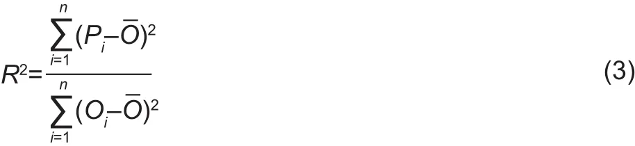

Where,PiandOiare the predicted and observed soil depth forith observation, respectively;nis the number of samples;are the means of the predicted and observed values, respectively;are the variances of the predicted and observed values, respectively;andris the Pearson correlation coef ficient between the predicted and observed values.
R2measures the matching of the linear relationship between the predicted and observed values. The closer theR2is to 1, the better the results are. LCCC provides a measure of how the predictions and observations adhere to a 1:1 relationship, where 1 corresponds to a perfect match between the predicted and observed values. ME indicates whether the model as a whole over- or under-predicted values (bias),whereas RMSE provides an indication of the prediction accuracy. Smaller ME and RMSE values indicate better model performances.
3. Results
3.1. Descriptive statistics of soil depth and environmental covariates
The basic statistics of soil depth and environmental covariates are summarized in Table 1. Soil depth varied from 0 to 200 cm with an average of 76.75 cm, and showed a moderately high correlation of variation, with a variance coef ficient of 63.59%. Based on the skewness coef ficient of 0.15,soil depth had a positively-skewed distribution. The complex landscape environment was re flected by the larger amplitude of variations of some environmental covariates and the significant discrepancies between the different covariates.
Pairwise coef ficients of correlation were computed to determine the significances of correlations between soil depth and quantitative predictors. Soil depth was positively correlated with B4 (r=0.50), NDVI(r=0.31), MAT (r=0.30), and Procur (r=0.25), and negatively correlated with elevation (r=–0.43), VDCN (r=–0.46), and Plancur (r=–0.23) (P<0.01 level). Soil depth was positively correlated with TWI (r=0.19) and B5(r=0.20), and negatively correlated with slope (r=–0.18) (P<0.05 level).The correlation coef ficients between environmental covariates were also computed. ELE and MAT, slope and TWI, and DI and MAP were negatively correlated at the 0.01 level, whereas B3 was positively correlated with NDVI and DI at 0.01 the level.
3.2. Different combinations of environmental covariates
Five combinations of environmental variables were derived based on different variable selection methods (Table 2).
As shown in Table 2, the number of variables in the combinations ofenvironmental covariates selected using the five methods varied significantly. The combination of cand_v contained the most variables (17), whereas IM_v contained the fewest (4). The combinations of PsCA_v, GAMs_v and RF_v contained the same number of covariates, and each contained topographic, climatic and biological factors. In contrast to IM_v, the climatic factor MAT and the topographic factors Procur and TWI were included in PsCA_v. The climatic factors MAP and MAT and the topographic factor cos_dN, which re flected the slope orientation, were included in GAMs_v. The climatic factors MAP and DI were included in RF_v.

Table 1Summary statistics of soil samples andenvironmental covariates1)
3.3. Performance of the different covariates combinations
Table 3 shows the prediction performances of soil depth using the five different covariates combinations (cand_v,PsCA_v, GAMs_v, RF_v, and IM_v) and two prediction methods (RF and SVM). The results show that the covariate combination IM_v from the proposed integrated method had better performance than the three conventional variable selection methods in terms ofR2and RMSE using either prediction methods. For the combination selected using only pedogenetic knowledge, the lowest prediction accuracy was obtained for the RF (R2=0.50, RMSE=19.52 cm) and SVM (R2=0.38, RMSE=37.56 cm) prediction methods.These comparisons of the prediction methods show that RF exhibited better prediction performance than SVM. Hence,we analyzed only the soil depth prediction results from the RF method below.
Of the three combinations selected using the conventional variable selection methods, GAMs and RF had better prediction accuracy than PsCA, and GAMs was slightly better than RF. This is because GAMs and RF consider the nonlinear relationships between the variables, whereas the variable selection of the PsCA method is based on the degree of linear correlation. Although the collinearity between the variables is considered in the PsCA method, it is insuf ficient to balance its inherent linear correlation basis.
TheR2values of the combinations of environmental variables fall in the range of 0.50–0.76. This indicates that for the combinations of the five selection methods, the model constructed using RF method can explain 50–76% of the variation in soil depth. Compared to other methods, the use of the integrated method to select the environmental variables resulted in an increasedR2(by 8–26%) and a decreased RMSE (by 2.25–7.64 cm). Furthermore, the prediction accuracy of soil depth was not affected by the number of variables.
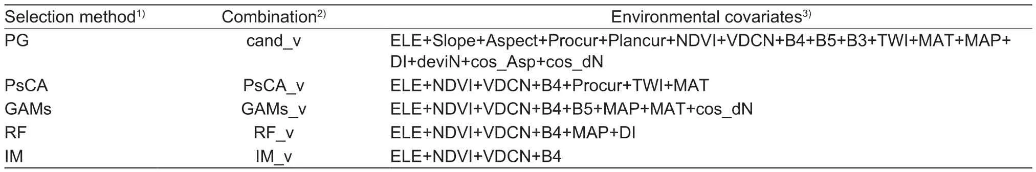
Table 2 Different combinations of environmental covariates

Table 3 Prediction performances of soil depth using the five different combinations and two prediction methods (Random Forest(RF) and support vector machine (SVM)1)
3.4. Spatial distribution and factors analysis of soil depth
The predicted soil depth obtained using the five variable selection combinations had similar spatial distributions over the entire area and had similar patterns in local areas, and the only differences were in the soil depth. Fig. 4 shows the regional and local spatial distributions of soil depth produced by the combination of covariates from the integrated method.In general, soil depth had a notably banded distribution at the regional scale. Thick soil was mainly distributed in hilly areas with gentle slopes and along the base of the Hexi Corridor in the southeastern part of the study area, whereas shallow soil was mainly distributed in glacial and canyon areas at high elevations as well as in areas with steep relief.The local distribution map shows that soil depth varied significantly with the topographic position, which suggests that high spatial variations of soil depth also occurred over relatively small areas.
Fig. 5 displays the differences in the prediction of regional and local distributions between the integrated method and the other variable selection methods. Table 4 summarizes the basic statistics of the differences in soil depth produced by the combinations of covariates from the integrated method and the other methods (PG, PsCA, GAMs and RF). As shown in Fig. 5 and Table 4, the integrated method and the pedogenetic knowledge method had the most significant differences in the prediction results (Fig. 5-A).The differences greater than 20 cm were mainly located in areas with relatively large topographic variations (such as piedmont floodplains and mountain ridges) along the river valleys in the southeastern part of the study area as well as in areas of relatively high elevations in the northwestern part of the study area, whereas the differences less than 10 cm were mainly located in relatively low alluvial-diluvial plains with gentle slopes as well as in glacier-covered areas.Similar spatial distributions of the differences occurred between the integrated method and the PsCA and GAMs methods (Fig. 5-B and C); the differences were less than 10 cm over most of the study area, and the differences greater than 20 cm occurred occasionally in mountain ridge areas with extremely steep terrain. Compared with the PsCA and GAMs methods, the differences between the integrated method and RF method were less than 10 cm in most of the study area (Fig. 5-D), and the differences greater than 20 cm are mainly located in the relatively steep areas at high elevations in the arid northwestern part of the study area and in the floodplains in the river valleys.
The standard deviation of 100 times of the soil depth predictions was used to represent the uncertainty of the predictions. Fig. 6 shows the standard deviation maps of the predicted soil depth produced by the different covariate selection methods. The uncertainties using the five variable selection methods showed notable spatial variations. As shown in Fig. 6-A, the standard deviations for the pedogenetic knowledge method fell in the range of 1.79–3.48 cm, with a mean of 2.40 cm, which indicated the highest uncertainty. As shown in Fig. 6-B–D, the mean standard deviation for the PsCA, GAMs and RF methods were 2.17, 1.98 and 2.13 cm, respectively. As shown in Fig. 6-E, the standard deviations for the integrated method fell in the range of 0.73–4.46 cm, which was the widest range of the five methods, but the mean standard deviation for this method was only 1.68 cm, which suggested that it had the lowest uncertainty in this area. In general, high uncertainties mainly occurred in areas with relatively large spatial variations along the main water systems, such as river valleys and mountain ridges. This may be because these areas experience external forces (e.g., topographic position and water flow) that result in large local variations in soil depth, which in turn result in relatively large differences among the prediction results.
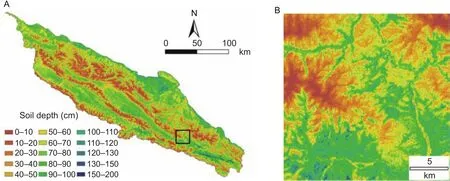
Fig. 4 Distribution map of soil depth (cm) derived from the combination of integrated method by using Random Forest. A, spatial distribution map of soil depth in regional area. B, small area outlined with black color in left large area for showing detail information.

Fig. 5 Maps of differences of the predicted soil depth between the integrated method (IM) and the conventional variable selection methods. A and E, difference distribution between the IM and pedogenetic knowledge (PG) method in regional and local areas.B and F, difference distribution between the IM and Pearson correlation analysis (PsCA) in regional and local areas. C and G,difference distribution between the IM and generalized additive models (GAMs) in regional and local areas. D and H, difference distribution between the IM and Random Forest (RF) in regional and local areas.

Table 4 Summary statistics of differences of the predicted soil depth between the integrated method (IM) and the conventional variable selection methods
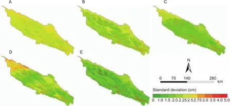
Fig. 6 Standard deviation maps of predicted soil depth (cm) produced by different variable selection methods. A, the pedogenetic knowledge method. B, Pearson correlation analysis. C, generalized additive models. D, Random Forest. E, the integrated method.
The relative importance of each covariate yielded by the RF method is shown in Fig. 7. Of the combinations of covariates obtained by PG, PsCA, GAMs, RF and IM, ELE was identi fied as the primary covariate affecting the spatial distribution of soil depth; it had a relative importance of 18.39, 30.31, 19.46, 18.26 and 32.15% in those methods,respectively. In addition, B4, NDVI and VDCN were dominant covariates that controlled distribution of soil depth.B5, MAP, MAT, and DI also affected the prediction accuracy of the corresponding methods. Of the aforementioned factors, ELE re flected the controlling effects of elevation on soil depth development in alpine areas; B4, NDVI and B5 mainly re flected the effects of surface vegetation conditions on soil depth; VDCN and Procur re flected the effects of regional water conditions and surface roughness on the development and redistribution of soil depth; and MAT,MAP and DI affected soil formation by changing the ambient temperature and humidity conditions.
4. Discussion
The combination of environmental covariates from the proposed integrated method explained more than 76% of the variation of soil depth, with an RMSE of 12 cm. Tesfaet al.(2009) selected variables based on the variable importance measured by the RF method in conjunction with correlation- filtered analysis to predict soil depth in a semiarid mountainous watershed. The results explained 31–52% of the variation in soil depth, and the RMSE for the calibration and testing data were 34 and 36 cm, respectively.Kuriakoseet al.(2009) selected variables using featurespace linear models with environmental predictors (LM) and predicted soil depth using LM and block regression kriging with the environmental predictors (BRK) method (R2=0.44 and RMSE=0.49 cm). Lacosteet al.(2016) predicted soil depth at a large regional scale. They selected environmental variables based on gradient boosting modeling (GBM) and predicted soil depth using three methods (including GBM).TheR2, RMSE, and LCCC values for the modeling sets fell in the ranges of 0.50–0.58, 35.66–39.76 cm and 053–0.73,respectively, in their three methods. In comparison, theR2values for all of the independent validation sets were the same (0.04), and the RMSE and LCCC for the independent validation sets fell in the ranges of 47–54 cm and 0.12–0.19,respectively. Li A Det al.(2017) derived seven topographic variables at a small watershed scale to predict active-layer soil thickness using RF (R2=0.62 and RMSE=10.85 cm),SVM (R2=0.49 and RMSE=12.67 cm) and other prediction methods. The results of this study show that the combination of covariates from the proposed integrated method has a relatively high prediction accuracy compared with the results of similar studies.

Fig. 7 Relative importance of each covariate as determined by Random Forest. PG, pedogenetic knowledge; PsCA,Pearson correlation analysis; GAMs, generalized additive models; RF, Random Forest; IM, the integrated method;ELE, elevation; deviN/cos_Asp/cos_dN, the transformations of Aspect; Plancur, plan curvature; Procur, pro file curvature;TWI, topographic wetness index; VDCN, vertical distance to channel network; MAT, mean annual temperature; MAP, mean annual precipitation; DI, drought index; B3, Landsat 5 TM band 3; B4, Landsat 5 TM band 4; B5, Landsat 5 TM band 5; NDVI,normalized difference vegetation index.
The predicted values of soil depth from the five variable selection methods had similar spatial distribution patterns.For example, thick soil is often distributed in low areas and areas with gentle slopes, whereas shallow soil is distributed in areas of high elevations or rugged relief. ELE, VDCN,NDVI, and B4 are the main environmental covariates that affect soil depth in the study area, and ELE is the most important covariate. The results obtained from this study,when combined with the results of previous research, can explain the spatial distribution of soil depth as well as the mechanisms of dominant covariates during the process of soil formation. Since the Holocene, the Qilian Mountainous area has been significantly affected by loess deposition,which is mainly affected by topographic factors, particularly elevation. Large amounts of loess have been deposited in low-elevations areas, which have resulted in the formation of thick soil masses. As elevation increases, the capacity of winds to transport and deposit dust decreases, which results in the deposition of relatively small amounts of loess at high elevations and, therefore, the formation of relatively thin soil masses in these areas (Nottebaumet al.2014, 2015). Moreover, as a result of the interaction of soil processes (soil erosion and soil deposition) and surface runoff, soil will migrate, settle and thus become redistributed,which results in variations in soil depth in areas with steep terrain or river valleys. Surface vegetation can effectively capture deposited matter, such as fallen dust, and facilitate soil accumulation (Pye 1995; Nottebaumet al.2015). On the other hand, climatic factors, such as MAT, MAP, and DI, were not selected as members of the covariate subset for predicting soil depth because climatic factors, such as temperature and precipitation, are significantly correlated with the elevation in mountainous areas (Körner 2003) and have relatively small impacts on the weathering of parent rocks and soil formation (Yanget al.2017).
In this study, the integrated method achieved the highest prediction performance with a relatively small number of covariates. In addition, the relatively small number of covariates not only reduces the running time of models but also facilitates understanding of model structure and interpretation of the relationships between the environmental covariates and soil attributes (Svetniket al.2003; Behrenset al.2010; Zhiet al.2017). However, the technical procedure of the integrated method is more complicated than that of conventional single-variable selection methods.We need to run several variable selection methods to obtain the corresponding optimal combinations and then perform a comprehensive process with these combinations to produce a final combination. Based on this study, we could develop a convenient variable selection tool for the proposed integrated method in the R language environment in the future. This tool should allow a set of original environmental variables to be used as input, and the covariate combination from the integrated method could be directly exported for use in digital soil mapping.
5. Conclusion
We propose an integrated variable selection method that is based on pedogenetic knowledge and several conventional selection methods. The effectiveness of the proposed method and other conventional methods (PsCA, GAMs,and RF) was evaluated through predictive mapping of soil depth. The prediction performance of the integrated method is significantly superior to other variable selection methods,and achieves the best prediction results with a relatively small number of predictor variables. This method improves the prediction accuracy of the model and is also able to satisfactorily explain the relationships between the genesis and development of soil depth and the environmental variables from the perspective of pedogenesis. Therefore,it is an effective variable selection method and provides a flexible framework to define combinations of environmental covariates for digital mapping of other soil attributes.
Acknowledgements
The study was supported financially by the National Natural Science Foundation of China (91325301, 41571212 and 41137224), the Project of “One-Three-Five” Strategic Planning & Frontier Sciences of the Institute of Soil Science,Chinese Academy of Sciences (ISSASIP1622), and the National Key Basic Research Special Foundation of China(2012FY112100). The authors wish to thank Yang Fan who comes from Chinese Academy of Sciences for the help of specifying the names of soil types.
杂志排行
Journal of Integrative Agriculture的其它文章
- Digital mapping in agriculture and environment
- Maize production under risk: The simultaneous adoption of off-farm income diversification and agricultural credit to manage risk
- miR-34c inhibits proliferation and enhances apoptosis in immature porcine Sertoli cells by targeting the SMAD7 gene
- lnhibition of KU70 and KU80 by CRlSPR interference, not NgAgo interference, increases the ef ficiency of homologous recombination in pig fetal fibroblasts
- Protective roles of trehalose in Pleurotus pulmonarius during heat stress response
- Kiwifruit (Actinidia chinensis) R1R2R3-MYB transcription factor AcMYB3R enhances drought and salinity tolerance in Arabidopsis thaliana