REGULARIZATION OF PLANAR VORTICES FOR THE INCOMPRESSIBLE FLOW∗
2018-11-22DaominCAO曹道珉
Daomin CAO(曹道珉)
Institute of Applied Mathematics,Chinese Academy of Science,Beijing 100190,China
E-mail:dmcao@amt.ac.cn
Shuangjie PENG(彭双阶)
School of Mathematics and Statistics&Hubei Key Laboratory of Mathematical Sciences,Central China Normal University,Wuhan 430079,China
E-mail:sjpeng@mail.ccnu.edu.cn
Shusen YAN(严树森)
Department of Mathematics,The University of New England Armidale,NSW 2351,Australia
E-mail:syan@turing.une.edu.au
Abstract In this paper,we continue to construct stationary classical solutions for the incompressible planar flows approximating singular stationary solutions of this problem.This procedure is carried out by constructing solutions for the following elliptic equations
Key words regularization;planar vortices;vorticity sets;reduction
1 Introduction
The following equations
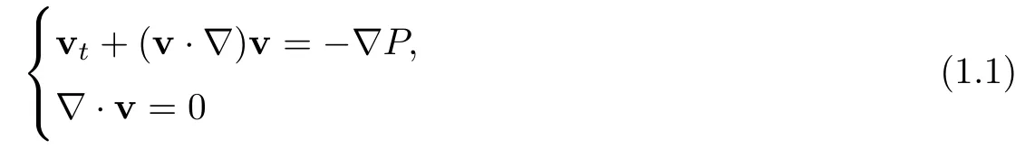
describe the evolution of the velocity v and the pressure P in incompressible flow.In a planar flow,the vorticity of the flow is de fined bywhich satis fies the equation

It follows from the second equation in(1.1)that for an incompressible steady planar flow,in any simply connected domain Ω,there is a function ψ,which is called the stream function of the flow,such that

Then the vorticity can be written as

We first discuss formally the equation involving with the vorticity ω
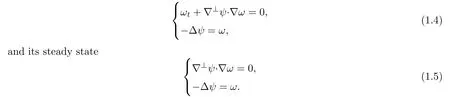
If ψ = ψ(y)and ω(y)= λf(ψ(y))for some function f,then

So,the first equation in(1.5)holds.
We remark that here λ is a positive constant which describes the strength of the vortex,f(u)is called the vorticity function in the context of fluid dynamics.
Set Γ(y)to be the Green function of−∆ in R2,that is,

and G(y,ξ)the corresponding Green function on Ω:
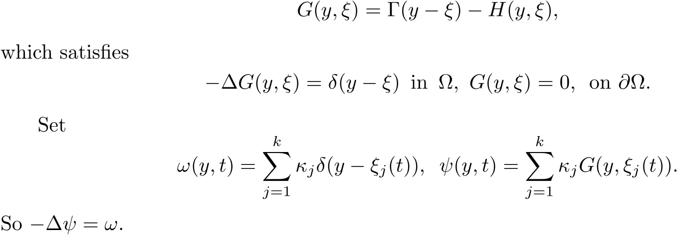
Formally we compute

Since Γ(y)and δ(y)are “radial”,we see

is the well-known Kirchho ff-Routh function(see[23]).In particular,critical point ξ of W corresponds to stationary singular vortex solution,which is exactly the Kirchho ff flow.In W,the parameters κjmay be positive or negative,which corresponds to the anti-clockwise or clockwise vortex motion of the flow at point ξjrespectively.As for the existence and multiplicity of critical point of W,we refer to[6]and the references therein.
The question on the existence of solutions representing steady vortex rings occupies a central place in the theory of vortex motion initiated by Helmholtz in 1858.There exist a great literatures dealing with the stationary impressible Euler equation.See for example[1–3,5,7,9,11–13,17,20,24,27–30]and the references therein.There are two commonly used methods to study the vortex problem,which are the stream-function method and the vorticity method.The vorticity method was first established by Arnold(a good reference is the book by Arnold and Khesin[4])and further developed by Burton[8,9],Amick and Fraenkel[2],Friedman and Turkington[20],Turkington[29,30].This argument was usually used in a constrained sublevel sets of ω to detect existence of the maximizer of the of the kinetic energy.
The stream-function method is to find a solution of(1.5),whose boundary condition can be homogenized as
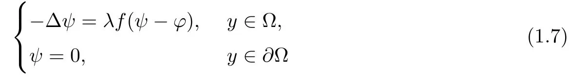
under the condition v ·ν =0 on ∂Ω,where ν is the unit outward normal of∂Ω.We point out that once we find the stream function ψ,the velocity of the flow is given by(1.3)and the pressure is given by

In(1.7),the vorticity function f(u)usually satis fies f(u)=0 if u≤0,the region{y∈Ω:f(uλ)> ϕ},which is called the vorticity set of the flow,is unknown(see[3,5,17,18,26]).Physically,f(u)is discontinuous,corresponding to a jump in the vorticity at boundary of the vortex ring.It is well known now that to find a solution for(1.7),one can use either a variational method such as the mountain pass lemma(see Ni[25]for instance),or a finite dimensional reduction argument.For the earlier work,we refer to the papers of Fraenkel and Berger[17]and Norbury[26,27].The advantage of a finite dimensional reduction argument,once it can be used,is that solutions concentrating at a saddle points,or concentrating at several points can be constructed[11,12,16].But if f(y,u)is not C1,it is very delicate to use the finite dimensional reduction argument even in the case that f(y,u)is continuous.See for example[12]in the construction of solutions for the plasma problem.If f(y,u)is C1and convex,the readers can refer to the results in[11,16,19,21,22,24,25,28,31]and the references therein.
A very interesting problem is to justify the weak formulation for point vortex solutions for the incompressible planar flow by approximating these solutions with classical solutions,which is called “regularization” of point vortices.A lot of work has been done in this respect,see[1,5,7,9,24–26,28,29]and the references therein.
For problem(1.7),a typical model is

where κ >0 is a constant,p≥ 0 is a number.For the superlinear case,i.e.,p>1,Li,Yan and Yang in[21]and Smets and von Schaftingen in[28]gave the exact asymptotic behavior and expansion of the least energy solution by estimating the upper bound of the energy.In[11],using a constructive argument,Cao,Liu and Wei proved the existence of a stationary classical solution approximating stationary multi-points convex solution.The case p=1 corresponds to the well-known plasma problem and was first studied by Ca ff arelli and Friedman in[10],where existence of solutions whose plasma set consists of one component and the asymptotic behavior of the plasma set for such solutions were investigated.In[12],the authors showed by a constructive method that problem(1.9)has solutions whose plasma set has multiple connected components if the homology of Ω is nontrivial.Recently,in[13],the authors studied the vortex patch problem in the planar flows,where p=0,i.e.,.There the authors proved the existence of a planar flow,such that the vorticity ω of this flow equals a large given positive constant λ in each small neighborhood of xi(i=1,···,k)and ω =0 elsewhere provided the Kirchho ff-Routh function W has a non-degenerated critical point in Ωk.Moreover,as λ → ∞,the vorticity set{y:ω(y)= λ}shrinks to
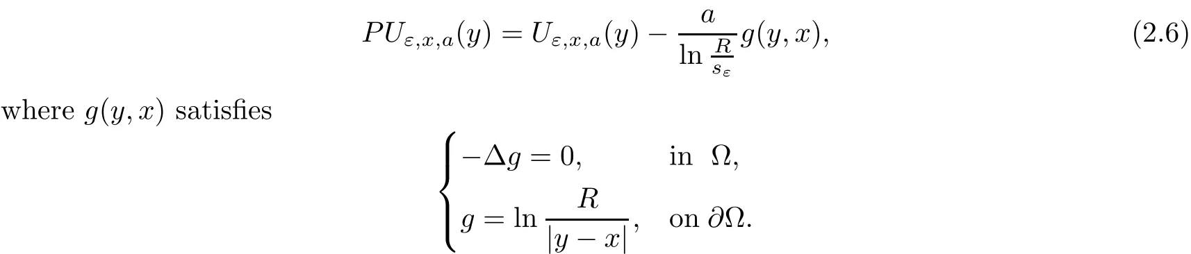
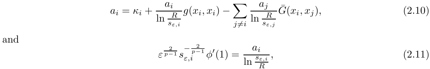
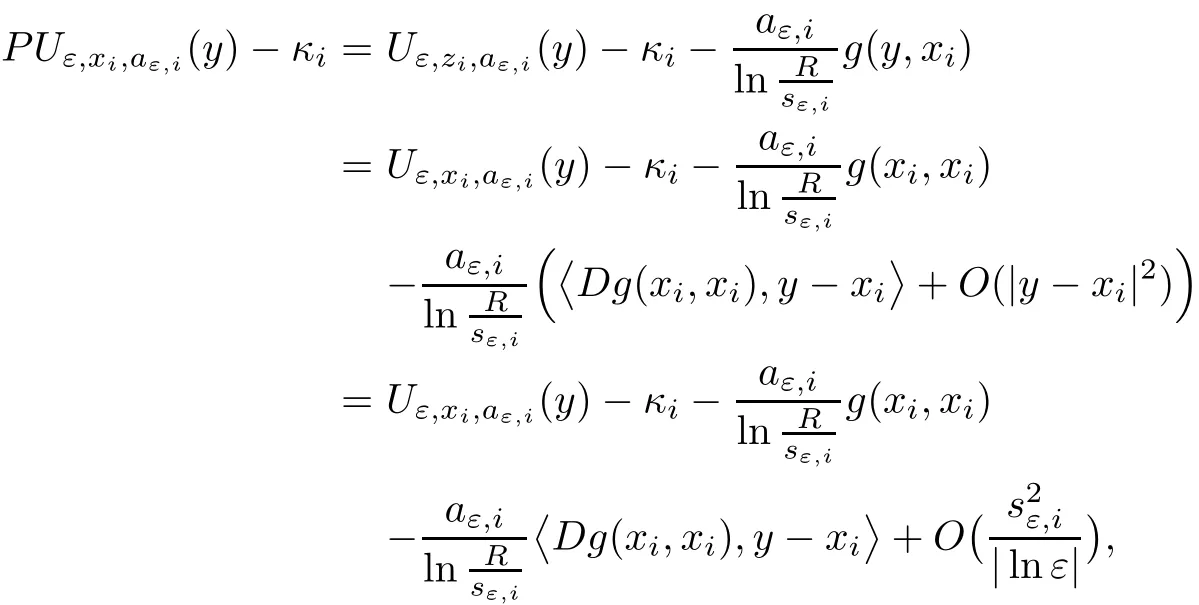
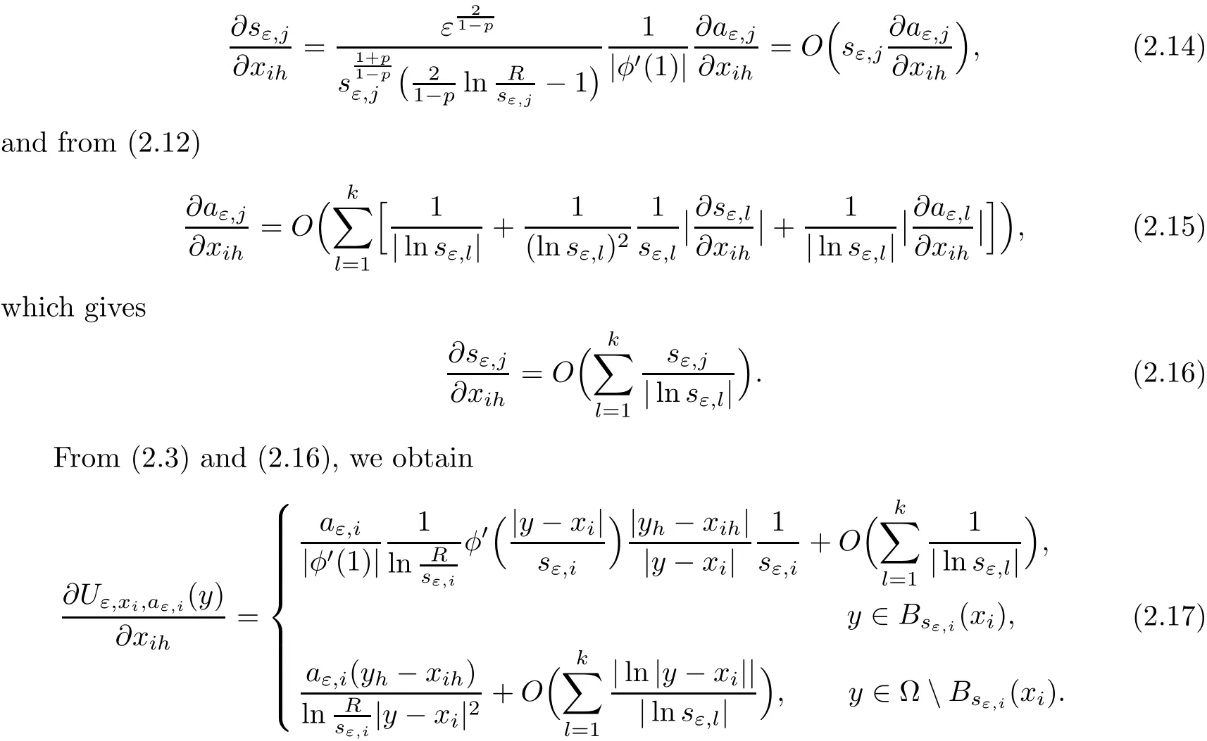
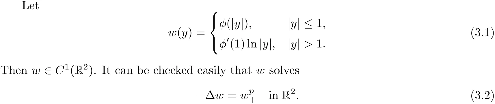
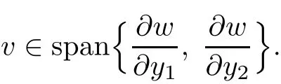
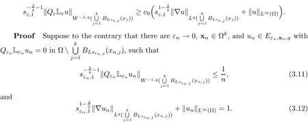
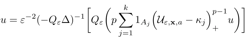
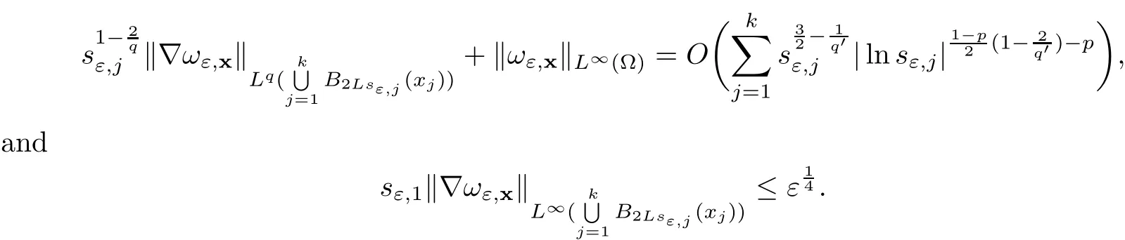
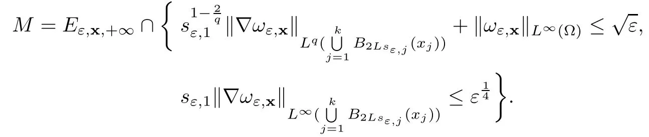
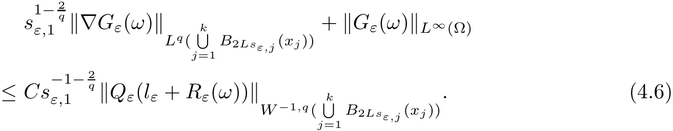
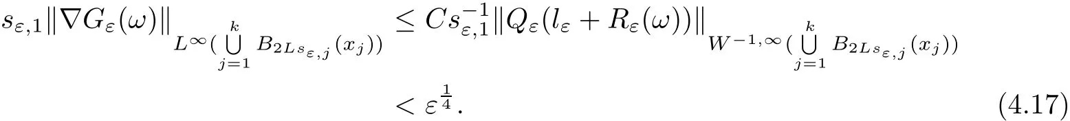
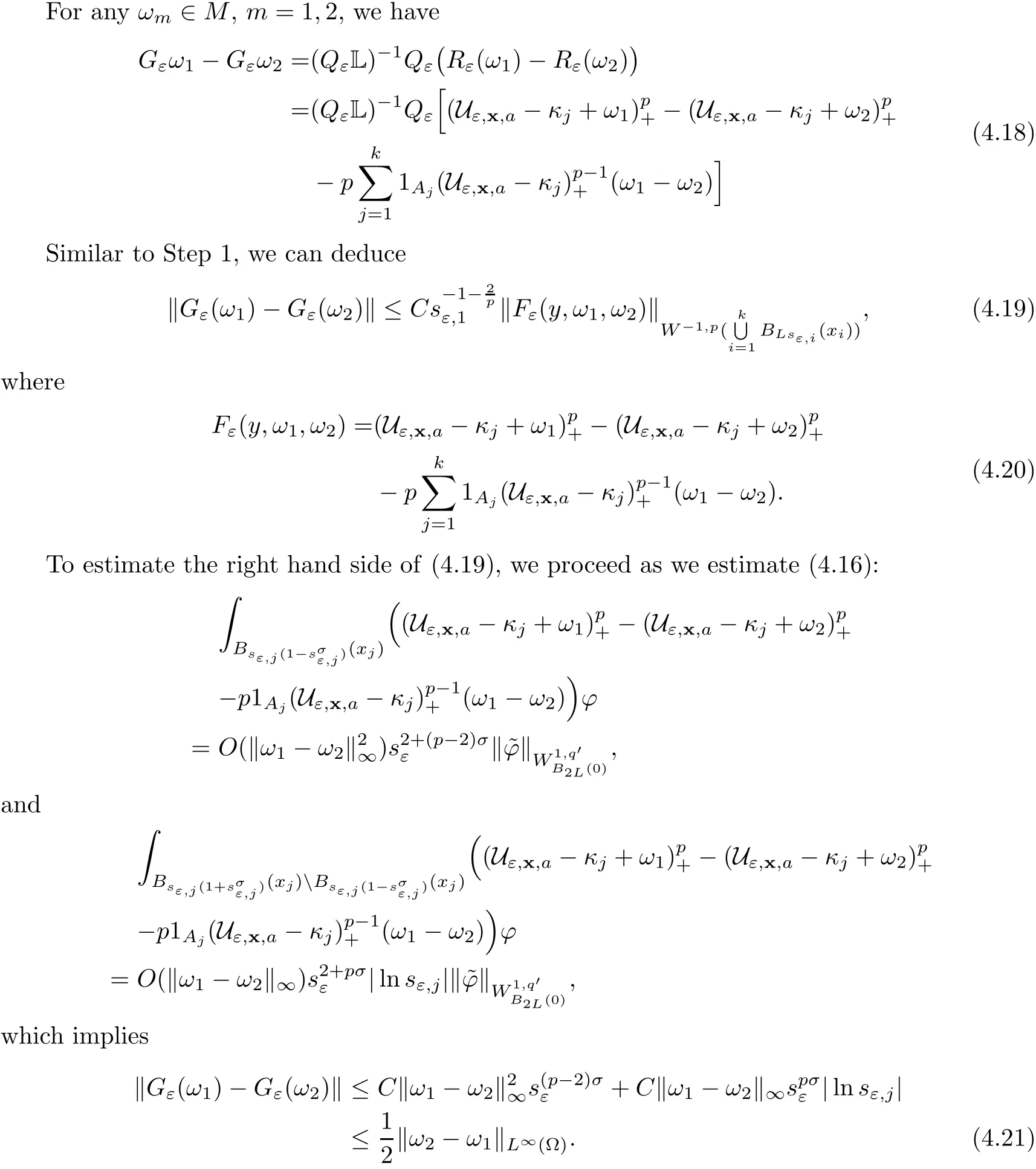
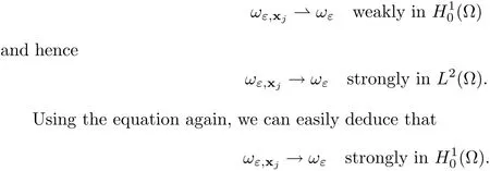
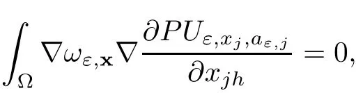
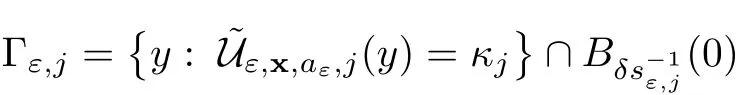
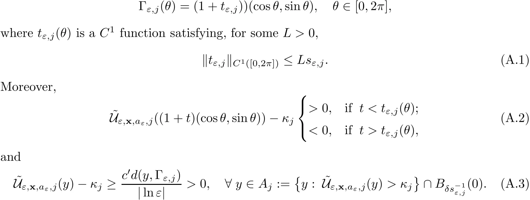
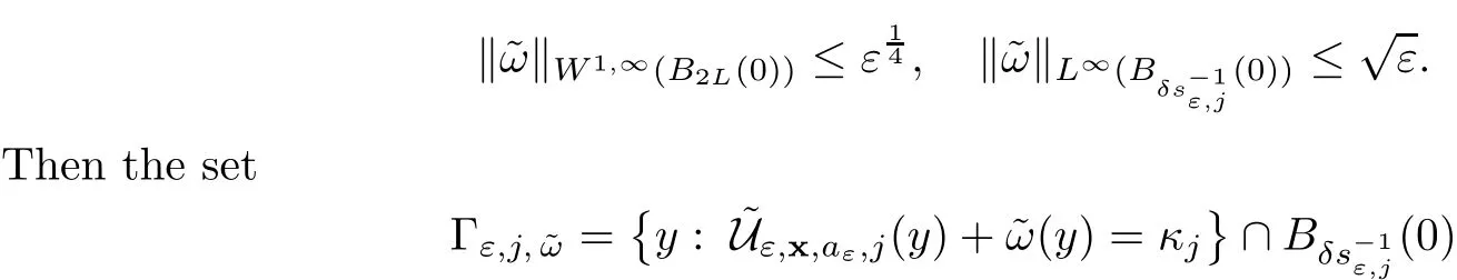
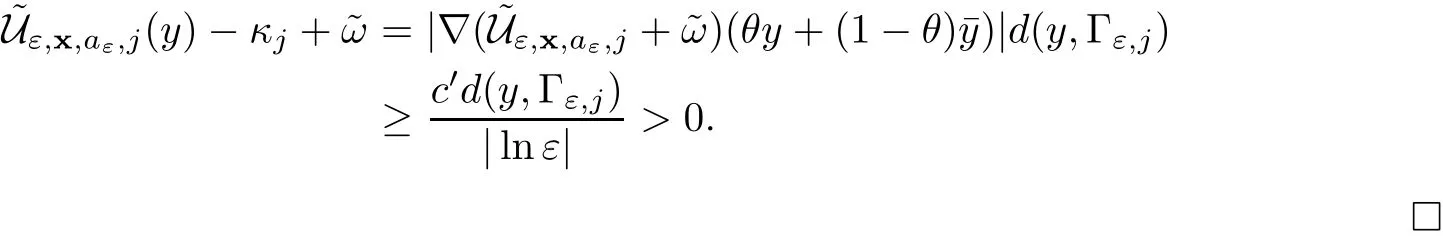
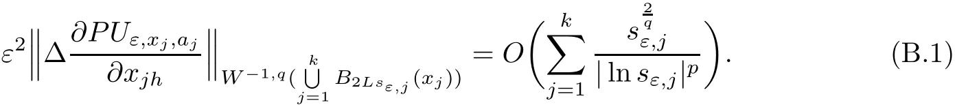
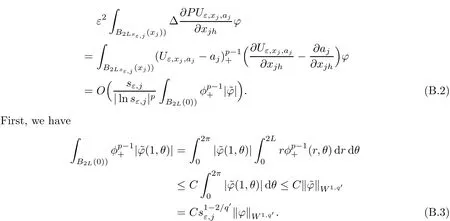
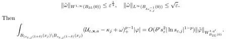
In the present paper,we will consider(1.9)for the sublinear case 0 where 0 Let the Kirchho ff-Routh function W be de fined by(1.6)(for simplicity,we denote H(y,y)by H(y)in the sequel).Note that if k=1,then W=κ2H. The main result of this paper is the following. Theorem 1.1Let κj,j=1,···,k,be k given positive numbers.Suppose that x0=(x0,1,···,x0,k)∈ Ωkis an isolated critical point of W(x)de fined by(1.6)satisfying deg(∇W,x0)6=0.Then,there is an ε0>0,such that for all ε∈ (0,ε0],(1.10)has a solution uεsuch that the vorticity set Ωε,i:={y:uε(y)− κj>0}shrinks to x0as ε→ 0. Remark 1.2It follows from the proof of the main result that,the vorticity set Ωε,i(i=1,···,k)satis fies preciselywhere L>0 is a give constant,xε,i→ x0,i(as ε → 0)and sε,isatis fies(2.5).Moreover,the vorticity on the vorticity set Ωε,itends to κias ε→ 0. To prove Theorem 1.1,although we use a finite reduction argument as in[11,12,16],we need to deal with some serious difficulties when the nonlinear term is sublinear.Mathematically,there is a striking di ff erence between the case p≥1 and 0 Remark 1.3As we have done in[12,13],our argument can also be used to study two other cases in planar point vortex problems.The first case is that the rotation of the flow at xifor some i ∈ {1,···,k}is clockwise.The second case is that the boundary of Ω is not the level set of the stream function ψ.In both cases,we obtain stream functions ψλ,whose vortex rings shrink to some prescribed points as λ → +∞. This paper is organized as follows.In Section 2,we will construct an approximate solution for(1.10)and study its properties,while in Section 3,we prove that the linearized operator corresponding to the approximate solution constructed in Section 2 is invertible in a suitable space.We will carry out a reduction procedure in Section 4 to reduce the problem of finding a solution for(1.10)to a finite dimensional problem.The proofs of Theorem 1.1 will be given in Section 5. In the section,we will construct an approximate solution for(1.10). Let R>0 be a large constant,such that for any x∈Ω,Ω⊂BR(x).First we take a radial solution φ for the following problem: For example,such a solution can be taken as a minimizer ofin the radial symmetric space Now we consider where a>0 is a constant.Then,(2.2)has a solution Uε,a,which can be written as where φ(y)is a radial solution of(2.1),and sεis the constant,such that Uε,a∈ C1(BR(0)).So,sεsatis fies We see that if ε>0 is small,(2.4)is uniquely solvable for sε>0 small.Moreover,we have the following expansion for sε: For any x ∈ Ω,de fine Uε,x,a(y)=Uε,a(y − x).Because Uε,x,adoes not satisfy the zero boundary condition,we need to make a projection.Let It is easy to see that where h(y,x)is the regular part of the Green function. Let x=(x1,···,xk)∈ Ωkbe a point close to x0,which is a non-degenerate critical point of the Kirchho ff-Routh function W de fined in(1.6).Denote and ajis chosen suitably close to κj. We will construct solutions for(1.10)of the form where ωεis a perturbation term. By(2.6),we have Since the estimate of the perturbation term ωεdepends on the terms on the right hand side of(2.9),to obtain a good estimate for ωε,we need to determine aε,jsuitably. Let aε,j(x)and sε,j,j=1,···,k,be the solution of the following problem: For simplicity,in this paper,we will use aε,iinstead of aε,i(x).Then we find that for y ∈ BLsε,i(xi),where L>0 is any fixed constant, and for j 6=i and y ∈ BLsε,i(xi),by(2.3) We now deduce some formulas which will be used in next section. Note that aε,jand sε,jdepend on x.It is easy to check from(2.4) Note that w>0 if|y|<1 and w<0 if|y|>1.Moreover,by the regularity theory,w∈C1,αfor any α∈(0,1). Now we consider the following problem where 1B1(0)=1 in B1(0)and 1B1(0)=0 in R2B1(0). Proposition 3.1Let v∈L∞(R2)∩C(R2)be a solution of(3.3).Then ProofThe proof is essentially similar to that of[16].Sinceis singular at r=1, some modi fications are needed. Letµjbe the eigenvalue of the Laplace-Beltrami operator on S1with corresponding eigenfunction ξj.Then,µ0=0,µ1= µ2=1 and µj>1 for j ≥ 3.For any solution v of(3.3),write Then,we find that vj(r)satis fies where r=|y|.Since v is bounded,we see that each vjis bounded.We claim that v0=0,vj=0 for j≥ 3 and vj=cjw′,j=1,2. First,with the standard argument(see[16],for example),we conclude that vj≡0 for j>2. Secondly,we prove v0≡ 0.Since v0is radial,∆v0=0 for|y|>1 and v0is bounded,we know that v0=c0for|y|≥1,and hence=0. Now we want to prove v0(1)=0.To this aim,multiplying the following equation by φ and integrating on B1(0), which,together with(3.6),implies v0(1)=0. Now we get v0(1)=0=.In the sequel,we want to conclude v0≡0.Unlike the smooth case,we can not use the uniqueness of solution for the initial value problem for ordinary di ff erential equations directly sinceis singular at r=1. Similarly,we can prove Finally,we consider the case j=1,2. Since w′is a bounded solution of and the other solution which is independent of w′is unbounded,we can easily check that there exists some cj>0 such that vj=cjw′for r>0. ? We intend to find a solution u=Uε,x,a+ω for(1.10).So,ω satis fies The operator Qεcan be regarded as a projection from W−1,q(Ω)to Fε,x,q.To prove the existence of bj1and bj2,we use(2.6)and(2.17)to find where δij=1 for i=j,but δij=0 for i 6=j.So(3.8)has a unique solution. Now we de fine the linear operator Lεas follows. We have Proposition 3.2For any q ∈ (2,+∞],there are constants c0>0 and ε0>0,such that for any ε∈ (0,ε],u ∈ Ewith QLu=0 in 0ε,x,qεεfor some large L>0,then Firstly,we estimate bn,jhin the following formula: It follows from Lemma A.1 that there exists large L>0 such that De fine For any function w,we denoteIt follows from Lemma A.1 that which,together with(3.18)gives Since the right hand side of(3.23)is bounded inis bounded inNoting that q>2,we deduce from the Sobolev embedding thatis bounded infor some α>0.So,we can assume thatconverges uniformly in any compact set of R2to u∈L∞(R2)∩C(R2).It is easy to check that u satis fies However,un=0 on ∂Ω and un=o(1)on ∂BLsεn,j(xn,j).By the maximum principle, So,we have proved that Moreover,it follows from(3.23)and the Sobolev embedding that for any ϕ∈C0(B2L(0)), Proposition 3.3QεLεis one to one and onto from Eε,x,qto Fε,x,q. ProofIf QεLεu=0,then Proposition 3.2 implies u ≡ 0.Thus,QεLεis one to one.Next,we prove that QεLεnis an onto map.Let By the Fredholm alternative,(3.31)is solvable if and only if has trivial solution.That is,QεLεis a one to one map. From Using Proposition 3.3,we can rewrite(4.1)as In this section,we reduce the problem of finding a solution for(1.10)to a finite dimensional problem. Proposition 4.1Fix a constant q>2.There is an ε0>0,such that for any ε∈ (0,ε0],(4.1)has a unique solution ωε,x∈ Eε,x,+∞,with Moreover,ωε,xis a continuous map from x to Eε,x,qin the norm of H1(Ω). ProofSet We will show that Gεis a contraction map from M to M. Step 1Gεis map from M to M. For any ω∈M,similar to Lemma A.2,it is easy to prove that Note also that for any u∈ L∞(Ω), Therefore,we can apply Proposition 3.2 to obtain It follows from(3.9)that the constant bjhin the following decomposition we find that the constant bjhin the decomposition in(4.7)satis fies On the other hand,from Lemma B.1, Using(4.8)and(4.9),we obtain As we estimate(3.15),de fine D1,D2as in(3.16).We see from(B.5) It follows from Lemma A.2 that there exists a small positive constant,denoted by σ>0,such that for and ω∈M,there holds but From Lemma A.1,we see that for y and from Lemma A.2,we see that for any Inserting(4.16),(4.13)and(4.10)into(4.6),we conclude that Similarly,choosing q=∞in the above analysis,we see Step 2Gεis a contraction map under the norm Note that M is closed in this norm. So Gεis a contraction map. Combining Step 1 and Step 2,we have proved that Gεis a contraction map from M to M.By the contraction mapping theorem,there is a unique ωε,x∈ M,such that ωε,x=Gεωε,x. Moreover,it follows from(4.13)that Finally,suppose that xj→ x0,then by(4.22),ωε,xis uniformly bounded in L∞(Ω)for all xj.Thus,we conclude thatand C is independent of xjbut depends on ε.Then there is a subsequence(still denoted by xj)such that Hence ωε∈ Eε,x0,pand ωεsatis fies(4.1)with x replaced by x0.By the uniqueness,ωε= ωε,x0and hence ωε,xis continuous in x in the norm of H1(Ω). ? In this section,we choose x,such that Uε,x,a+ ωε,xis a solution of(1.10),where ωε,xis the map obtained in Proposition 4.1, The next result shows how to choose x: Lemma 5.1If x satis fies for j=1,···,k,h=1,2,then Uε,x,a+ ωε,xis a solution of(1.10). ProofProposition 4.1 with(5.1)implies Now we need to solve(5.1). Lemma 5.2(5.1)is equivalent to ProofNoting that we can proceed as we estimate(4.11)to derive where σ >0 is a small constant.Here,we have used thatfor i 6=j. Noting that aε,i→ κi,we conclude the result. Proof of Theorem 1.1By our assumption,from Lemma 5.2,(5.2)has a solution xεsatisfying xε→ x0as ε→ 0. By our construction,we find Appendix A The Estimates for the Level Curves For any function w,for each j,we denoteThe following lemmas can be proved by the similar arguments to[13]and we omit it here. Lemma A.1The set is a closed curve in R2,which can be written as ProofThe proof of(A.1)and(A.2)can be found in[13]and we omit it.To prove(A.3),we need to prove it for y close toThen by the mean value theorem,there is a θ∈(0,1),such that Similarly,we can prove Lemma A.2Suppose thatis a function,satisfying is a continuous closed curve in R2,and As a consequence,is a continuous closed curve in R2. LetThen by the mean value theorem,there is a θ∈(0,1),such that Appendix B Some Essential Estimates Lemma B.1We have ProofRecall that φ is a radial solution of(2.1).We have On the other hand,in view ofwe find So the result follows. Lemma B.2Suppose that˜ω is a function,satisfying ProofWe use the same notations as in Lemma A.2.We have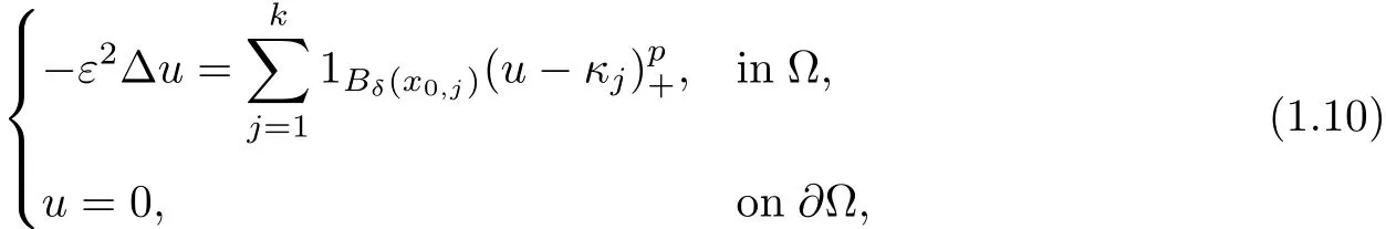
2 Approximate Solutions


3 The Linear Operator


4 The Reduction


5 Proof of the Main Results


杂志排行
Acta Mathematica Scientia(English Series)的其它文章
- YAU’S UNIFORMIZATION CONJECTURE FOR MANIFOLDS WITH NON-MAXIMAL VOLUME GROWTH∗
- STABILITY OF STEADY MULTI-WAVE CONFIGURATIONS FOR THE FULL EULER EQUATIONS OF COMPRESSIBLE FLUID FLOW∗
- ONE-DIMENSIONAL VISCOUS RADIATIVE GAS WITH TEMPERATURE DEPENDENT VISCOSITY∗
- MACROSCOPIC REGULARITY FOR THE BOLTZMANN EQUATION∗
- RADIAL SYMMETRY FOR SYSTEMS OF FRACTIONAL LAPLACIAN∗
- STRONG COMPARISON PRINCIPLES FOR SOME NONLINEAR DEGENERATE ELLIPTIC EQUATIONS∗