Statistical description of depth-dependent turbulent velocity measured in Taihu Lake,China

Lin Yuan,Hong-guang Sun,*,Yong Zhang,Yi-ping Li,Bing-qing Lu

aState Key Laboratory of Hydrology-Water Resources and Hydraulic Engineering,Hohai University,Nanjing 210098,China

bCollege of Mechanics and Materials,Hohai University,Nanjing 210098,China

cDepartment of Geological Sciences,University of Alabama,Tuscaloosa,AL 35487,USA

dCollege of Environment,Hohai University,Nanjing 210098,China

Abstract Quantitative description of turbulence using simple physical/mathematical models remains a challenge in classical physics and hydrologic dynamics.This study monitored the turbulence velocity field at the surface and bottom of Taihu Lake,in China,a large shallow lake with a heterogeneous complex system,and conducted a statistical analysis of the data for the local turbulent structure.Results show that the measured turbulent flows with finite Reynolds numbers exhibit properties of non-Gaussian distribution.Compared with the normal distribution,the Lévy distribution with meaningful parameters can better characterize the tailing behavior of the measured turbulence.Exit-distance statistics and multiscaling extended self-similarity(ESS)were used to interpret turbulence dynamics with different scale structures.Results show that the probability density function of the reverse structure distance and the multiscaling ESS can effectively capture the turbulent flow dynamics varying with water depth.These results provide an approach for quantitatively analyzing multiscale turbulence in large natural lakes.

©2018 Hohai University.Production and hosting by Elsevier B.V.This is an open access article under the CC BY-NC-ND license(http://creativecommons.org/licenses/by-nc-nd/4.0/).

Keywords:Finite Reynolds number turbulence;Reverse structure function;Lévy distribution;Probability density function;Multiscaling extended self-similarity(ESS)

1.Introduction

Lakes are among the major global freshwater resources,with hydrologic properties such as turbulent flows that can affect sediment dynamics and aquatic system evolution.Presently,pollutants discharged from lakes far exceed the self renewal capacities of lake water,resulting in various environmental problems.One of the main causes is the indigenous nutrient release from the bottom of shallow lakes(Wetzel,2001).Suspended sediment can interact with nutrients through adsorption and desorption(Chao et al.,2008).Windinduced currents and waves have been found to dominate sediment transport and resuspension in shallow lakes(Csanady,1973;Liang and Zhong,1994;Han et al.,2008;Chen et al.,2012).Many studies have focused on basic processes of sediment transport,such as sediment resuspension under the impact of flow circulation(Jin and Sun,2007),sediment transport due to wind-induced wave action(Luettich et al.,1990;Hawley and Lesht,1992),and deposition(Mehta and Partheniades,1975).However,the sediment resuspension process is the direct result of the disturbed vertical velocity.From this perspective,macroscopic analysis and description of sediment,without reliable exploration of the small-scale velocity structure,may not be sufficient to characterize the resuspension dynamics.Due to the complexity of natural lakes,standard statistical analysis may be inadequate to explain the mechanism of natural processes.Novel statistical analysis methods are needed to identify velocity fluctuations in turbulence(Frisch,1995)and interpret real environmental processes.

Turbulence is a flow regime with multi-scale chaotic changes in pressure and flow velocity(Holmes et al.,1998;Tabeling,2002;Stull,2012;Davidson,2015).However,we do not yet have a physical understanding of real turbulence,or a well developed manner of statistically describing it(Feynman et al.,1966;Nelkin,1992;ˇSvihlová et al.,2017).In traditional statistical analysis,turbulence is often regarded as a random field,and a structure function is used to describe its statistical characteristics.Kolmogorov(1968)proposed a structure function describing the local turbulent structure based on dimensional analysis,and found that the velocity of aflow particle in homogeneous isotropic turbulent flow with a sufficiently high Reynolds number(i.e.,developed turbulence)in the inertial sub-region satisfies ul= （εl）1/3,where ulis the velocity,ε is the turbulence dissipation rate,and l is the scale.The structure function means that the velocity difference of the fluid particle satisfies the following scaling law:

where δu（r）represents the velocity difference between two points x and x+r,with r being the spatial distance,and δu（r）=u（x+r）-u（x）;p is the order;ξ is the scaling index;and 〈·〉represents the ensemble average.According to the structure function,Kolmogorov(1941)proposed the K41 similarity assumption:ξ（p）=p/3,corresponding to the inertial-region scaling law.

When describing the small-scale statistical characteristics of turbulence,the inertial-region scaling law is strictly true only if the Reynolds number tends to infinity.In actual turbulence,the existence of coherent structures leads to the intermittent instantaneous turbulent energy consumption(Douady et al.,1991;Vincent and Meneguzzi,1991;Liu and Jiang,2004),indicating that there is an essential difference between the real turbulent flow field and the completely random field in Kolmogorov(1941).The movement of a particle in turbulence is affected by the corresponding turbulence structure,and the motion of the fluid mass is not completely random(Liu and Jiang,2004).At this time,due to the nonlinear scaling feature of the structure function,the scaling structure in the turbulent inertial region exhibits different scaling features,and the K41 similarity assumption is not suitable for real turbulence.

In view of the complexity of the actual turbulence structure,Jensen(1999)proposed a reverse method to describe and analyze the turbulent velocity field,and defined a reverse structure function to explore the scaling relation:

where r（δu）is the reverse structure distance,also called the exit distance,which is defined as the minimum distance between two fluid masses with velocity difference exceeding δu;and ζ（p）is the exit-distance order,also known as the inverse statistical order.According to the K41 hypothesis,the scaling relation of the inverse structure function can be obtained theoretically: ζ（p）=3p(Jensen,1999).However,the results obtained from the actual turbulence model do not reflect a similar relationship(Frisch,1991).Therefore,the study of turbulence reverse structure functions is far from perfect.There are many studies and applications focusing on reverse statistical analysis.For example,Biferale et al.(2001)provided numerical evidence that the reverse structure analysis of two-dimensional turbulent flows can reveal a rich multiscale structure.Viggiano et al.(2016)used the inverse structure functions to study the statistical properties of canonical wind turbine array boundary layer flow.Zhou et al.(2006)found that the statistical functions of exit distances can be approximated by stretched exponentials.

In natural sciences,many complex behaviors and phenomena are widely distributed at spatiotemporal scales,which can be quantified by a non-Gaussian probability density function(PDF)within a given scale range(Frisch,1995).In turbulence,the Lévy stable distribution (Uchaikin and Zolotarev,1999;Nolan,2003)completely solved the question of scaling and the paradigm of fractals,and dealt with the divergence of high-order moments of the PDF(Shlesinger et al.,1987).The Lévy stable distribution has four parameters:the stability index α (0 ＜ α ≤ 2),skewness parameter β(-1＜ β ＜ 1),scale parameter γ (γ ＞ 0),and location parameter δ (δ∈ R).When α =2 or α =1,the Lévy stable distribution reduces to a Gaussian distribution or Cauchy distribution,respectively.Nolan(2003)summarized statistical characteristics of Lévy distribution.Studies of turbulence have found that these non-Gaussian physical quantities obey Lévy stable distributions(Chen and Zhou,2005).Moreover,the Lévy stable distribution has been widely applied to the statistical-mechanical description of dynamic turbulence systems,such as Lévy flight(Feller,2008),random processes based on Lévy stable distributions,and Lévy walks(Shlesinger et al.,1987),which are random walks with a nonlocal memory coupled in space and time in a scaling fashion.We propose a Lévy stable distribution to provide insight into the power law probability distribution of the disturbed vertical velocity.

In this study,the method of turbulence theory was used to analyze the non-Gaussian property and reverse structure function for turbulence,focusing on the turbulent flow field with a finite Reynolds number in a real scenario.Statistical analysis were conducted for the turbulent velocity with a finite Reynolds number in the surface and deep layers of Dongtaihu Bay(detailed information can be found in Li et al.(2017)).The velocities measured in both layers were analyzed in this study.Hu et al.(2010)found that the water transfer/renewal rate in Dongtaihu Bay is one-tenth of the average water transfer rates in Taihu Lake.Hence,it is necessary to study water transfer rates,which can be done by investigating the vertical profile.The disturbed vertical velocity in Dongtaihu Bay was measured using an acoustic Doppler current profiler(ADCP),an ultra-precise instrument,and velocity structures in different flow layers were evaluated.The rest of this paper is organized as follows:We first analyze the fluctuation values of the turbulent flow velocity statistically and then identify the non-Gaussian properties of the distribution.Next,we examine the flow velocity using the reverse structure function,and analyze different turbulence layer distributions at distances r with different δu values.Finally,based on the multiscaling extended self-similarity(ESS),we analyze the characteristics of the turbulence velocity scale law in different flow layers with a finite Reynolds number.

2.Observation of turbulent flow velocities in surface and deep layers in Taihu Lake

Two time series datasets were considered.They were measured in the surface and deep layers in the east bay of Taihu Lake.Taihu Lake is located southeast of the Yangtze River,near Wuxi City of Jiangsu Province.It is the third largest freshwater lake in China,with an area of 2338 km2and an average depth of 1.9 m.The surface area of Dongtaihu Bay is 131 km2,about 97%of which is covered by macrophytes(Qu et al.,2001).The three-dimensional instantaneous velocity(at a depth of 40 cm)was measured by an ADCP(Argonaut-XR,SonTek company,USA)at 8:00-16:00 on 25-27 May,2015,and the mean value was-0.0256 cm/s.The deep instantaneous velocity(at a depth of 195 cm)was measured using an acoustic Doppler velocimeter(ADV)Ocean(ADV SonTek company,USA)(5 MHz)at 8:00-16:00 on 25-27 May,2015,and the mean value was-0.0537 cm/s.An ADCP Argonaut-XR standard pressure sensor measured the depth of deployment and surface elevation automatically,to ensure that the measurement point was adjusted with water fluctuations and that the water depth remained fixed.More details on instrument and data collection can be found in Li et al.(2017).During the monitoring period,Dongtaihu Bay in the Taihu Lake Basin was dominated by cloudy weather with an average daily temperature of 23°C.Due to its geographical location,the wind speed was relatively slow,maintaining three-grade southeast wind.

3.Non-Gaussian property of spatial statistical distribution

Statistically,turbulence is considered a stationary stochastic process.Previous studies have used Langevin dynamic synthesis of multiple self-similar fields,considering the correlation between units,and found that the developed turbulence deviates from a Gaussian distribution to a very small extent(Ma and Hu,2004).Many natural phenomena show complex fluctuations in space and time scales.This complexity is characterized by a very uneven distribution of instantaneous turbulent energy consumption in time and space for finite Reynolds number turbulent flow,often referred to as an intermittent phenomenon.This phenomenon has been proven to be a non-Gaussian property of the PDF,which is reflected by the peak and tail of the PDF(Biferale et al.,2003).The tail of the non-Gaussian distribution shows violent fluctuations,which are the result of three-dimensional turbulent flow accompanied by intermittent flow and violent fluctuations.The peak of the PDF is linked to the laminar fluctuations,for example,smooth changes in the flow field.

As mentioned above,Lévy stable distributions are a general term for a class of distributions(Weron,2004),where the Gaussian distribution is a special case when α=2.The characteristics of sharp peak and heavy tail(or tailing)of the statistical distribution are shown at 0＜α＜2.There is a close intrinsic relation between the fractional Laplacian operator and the Lévy distribution.The Lévy distribution is often used as the statistical solution for the following fractional Laplacian Navier-Stokes(N-S)equation;that is,the fractional Laplacian operator is used to represent the cohesive effect of the finite Reynolds number turbulence(Chen and Zhou,2005):

where~Re is the Reynolds number related to α,t is the time,P1is the pressure,and Δ is the Laplacian operator.When α =2,Eq.(3)turns into the standard N-S equation.As mentioned above,the cohesive effect of the finite Reynolds number turbulence can be expressed by the stability index of the Lévy distribution when 0＜α＜2.

A new MATLAB toolbox(Liang and Chen,2013)was used to estimate the parameters of the Lévy distribution for turbulent flow velocities in surface and deep layers.In Fig.1,the Lévy distribution and the normal distribution are fitted to the empirical distributions of the turbulent flow velocity in the deep layer.The fitting results are expressed in Cartesian coordinates in Fig.1(a)and semi-logarithmic coordinates in Fig.1(b).The PDF distribution of the turbulent flow velocity in the surface layer is described in Fig.2.

The stability index of the Lévy distribution fitted by the turbulent flow velocity in the deep layer is α1=1.85,and the best-fit stability index using the near surface velocity is α2=1.79,indicating that the random velocity at different depths follows the heavy-tailed non-Gaussian distribution.Here the physical meaning of the heavy-tailed distribution refers to high velocities in the flow field with a low probability but a large impact on the transport of materials(carried by the water).Combination of the results with Eq.(3)shows the turbulent viscosity with a finite Reynolds number.The peak of the flow velocity distribution is different for different layers of the turbulence field.As shown in Fig.1,the velocity PDF in the deep layer has an obvious sharp peak and heavy tails,and it is well fitted by the Lévy distribution.Meanwhile,in Fig.2 the middle part of the velocity PDF in the surface layer conforms to the normal distribution,and the tails exhibit a power law trend deviating from the exponential distribution,indicating that the velocity fluctuation is depth-dependent.The sharp peak and heavy tails in the deep layer show that,in Taihu Lake,a large-scale shallow-water lake,the impact of the wind speed on the characteristics of water mobility is limited,and turbulence may mainly originate from the river bed and tend to decrease upward from the bottom.The heavy-tailed characteristics of the PDF distribution indicate that the extreme value of the flow velocity occurs with a certain probability,which significantly influences the resuspension of the nutrients in the bottom layer.

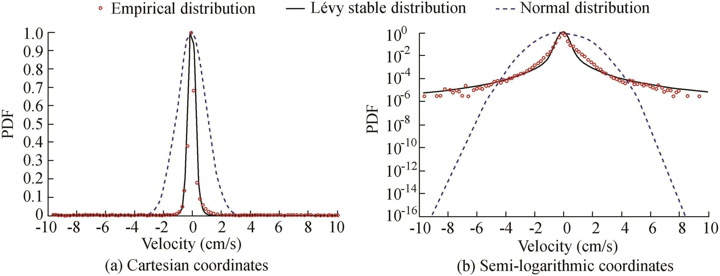
Fig.1.PDF of velocity in deep layer.

4.PDF of reverse structure distance for turbulent velocity of different layers with different δu and distance r

The PDF(P（r）)of the reverse structure distance for the velocity of the surface and deep layers can be regarded as a function of r/σ:

where σ = 〈|r|〉.We calculated the PDF of the reverse structure distance for three sets of velocity data with four different speed difference values: δu=0.05 cm/s, δu=0.10 cm/s, δu=0.15 cm/s,and δu=0.20 cm/s(Fig.3).The different colors represent the measurement arrays at different times t1,t2,and t3.The reverse structure distance r of the complete random turbulence velocity is irrelevant(corresponding to Poisson's statistics).However,for our measured turbulent flow velocity with a finite Reynolds number,the distribution of P（r）has a non-exponential tailing behavior,and follows a stretched exponential distribution.

Assuming n=r/σ,there is the following stretched exponential distribution(Zhou et al.,2006):

where m is the stretched exponent(0≤m≤1),and the parameters A and B are independent of speed difference values.The graph of Φ（n）versus n is characteristically stretched.When m=1,the standard exponential function is recovered,representing an irrelevant characteristic(corresponding to Poisson's statistics).The compressed exponential function(m＞1)has less practical importance,with the notable exception of m=2,which gives the normal distribution,and the specific case of m→0,which gives the power law distribution.More statistical characteristics of stretched exponential distribution can be found in Laherrere and Sornette(1998).The least square method is used to fit the data,and the results are shown as the solid lines in Fig.3.It can be seen from Fig.3(a)that P(r)shows strong independence from δu,tending to the same distribution for different δu values.Different measurement times did not have obvious impacts on P(r),indicating that P(r)is independent of time.

There is a significant difference between P(r)of turbulent velocities in the deep layer and that in the surface layer.P(r)of the velocity in the deep layer is depicted in Fig.3(b),showing a strong dependence on δu and time.P(r)for the large r agrees with a stretched exponential function,while the distribution curve of P(r)exhibits a deviation from the stretched exponential distribution at a small r and tends to be a power-law distribution(which is linear in log-log plots).In addition,we found that,with an increase in δu,the corresponding P(r)tends to be a power-law distribution.Bogachev et al.(2008)concluded that the probability distribution of distance r is close to a power-law distribution,which means that the velocity data have multifractal properties.The physical interpretation of this phenomenon is that the complexity and randomness of the velocity structure in the deep layer are higher than those in the surface layer.For the surface layer,P(r)of reverse structure distances is fully described by δu.Conversely,P(r)of reverse structure distances in the deep layer strongly depends on both δu and measurement time.

Fig.2.PDF of velocity in surface layer.

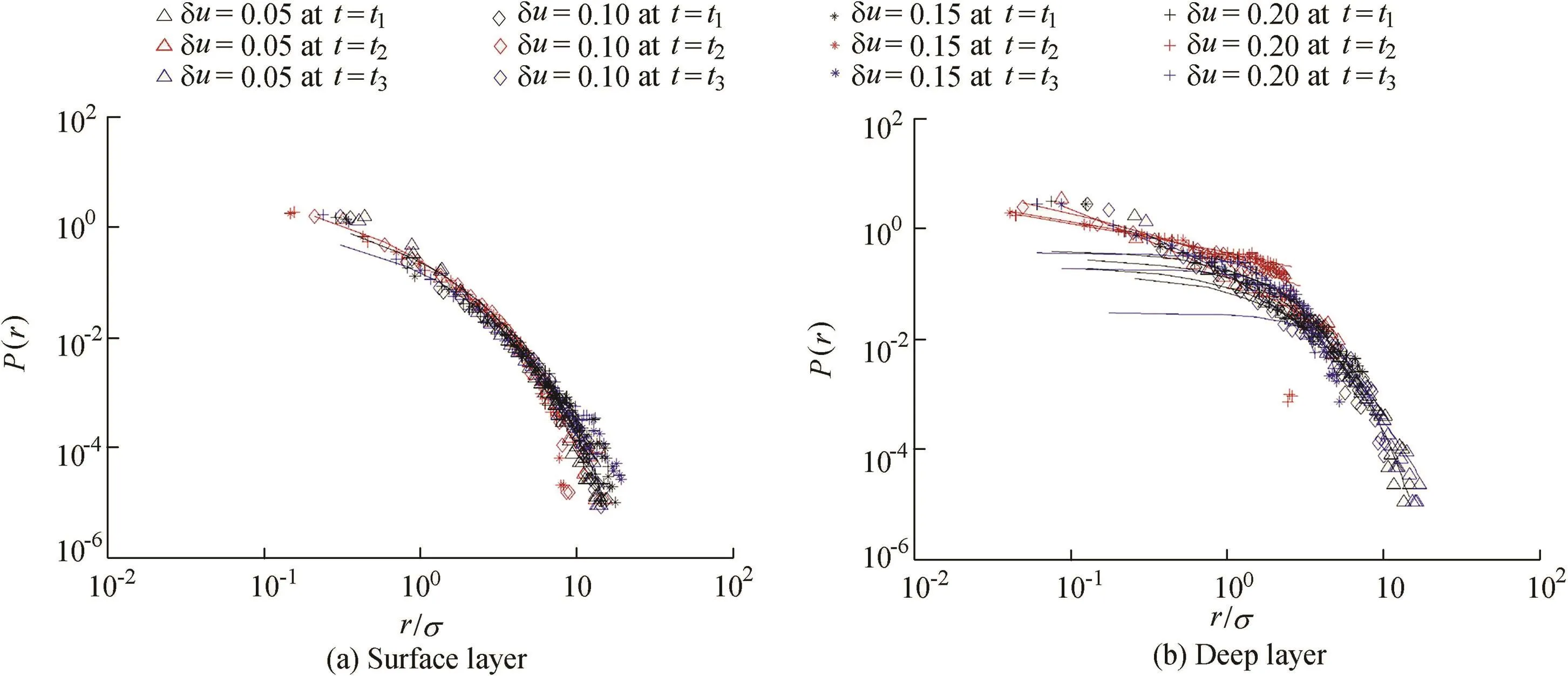
Fig.3.Probability density distribution of reverse structure distance for velocity in different layers.

5.ESS scaling law

The ESS method proposed by Benzi et al.(1993)was used to establish scaling properties of the reverse structure distance in turbulence with finite Reynolds numbers.If Tp（δu）=〈|r（δu）|p〉,we can obtain

where τ（p，p）is the relative scaling exponent,which is the slope of the double-logarithmic plot of Tp（δu）against Tp（δu）.

In this study,p=2 was used to calculate the scaling exponent for reverse structure distance.The multiscaling phenomenon of the velocity of turbulent flow with a finite Reynolds number in different flow layers is revealed in the wider scaling region provided by ESS.Based on a set of data,Fig.4 shows the double-logarithmic plot of Tp（δu）against T2（δu）at p=1，2，…，10，δu∈[0.03，0.20].There is a linear relationship between the reverse structure distance data derived from the selected velocity difference δu at different orders,indicating that there is an ESS scaling law.It is noteworthy that the scaling relationship between different orders reflects the multiscaling behavior of the flow velocity structure.

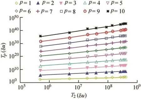
Fig.4.Relationship between Tp（δu）and T2（δu）

We calculated the ESS scaling exponent τ（p，2）for multiple sets of velocity data measured in deep and surface layers.The results are shown in Fig.5,where S represents the deep layer,and B represents the surface layer.Numbers correspond to different measurements of flow velocity groups.According to the K41 scaling law,we estimated the single scaling trend in the surface and deep layers,respectively,and obtained these results: τB（p，2）=0.59p,and τS（p，2）=0.45p,where τB（p，2）and τS（p，2）are the ESS scaling exponents in the surface and deep layers,respectively.These results show that there is a significant and quantifiable difference between the velocity scaling law ranges of the two different flow fields.Due to the influence of the actual complex environment,the difference between flow velocity structures causes the singularity of the scaling law,which is expressed as the scaling exponent τ.However,the effect of the finite Reynolds number does not deny the K41 normal scaling law(Qian,2001).

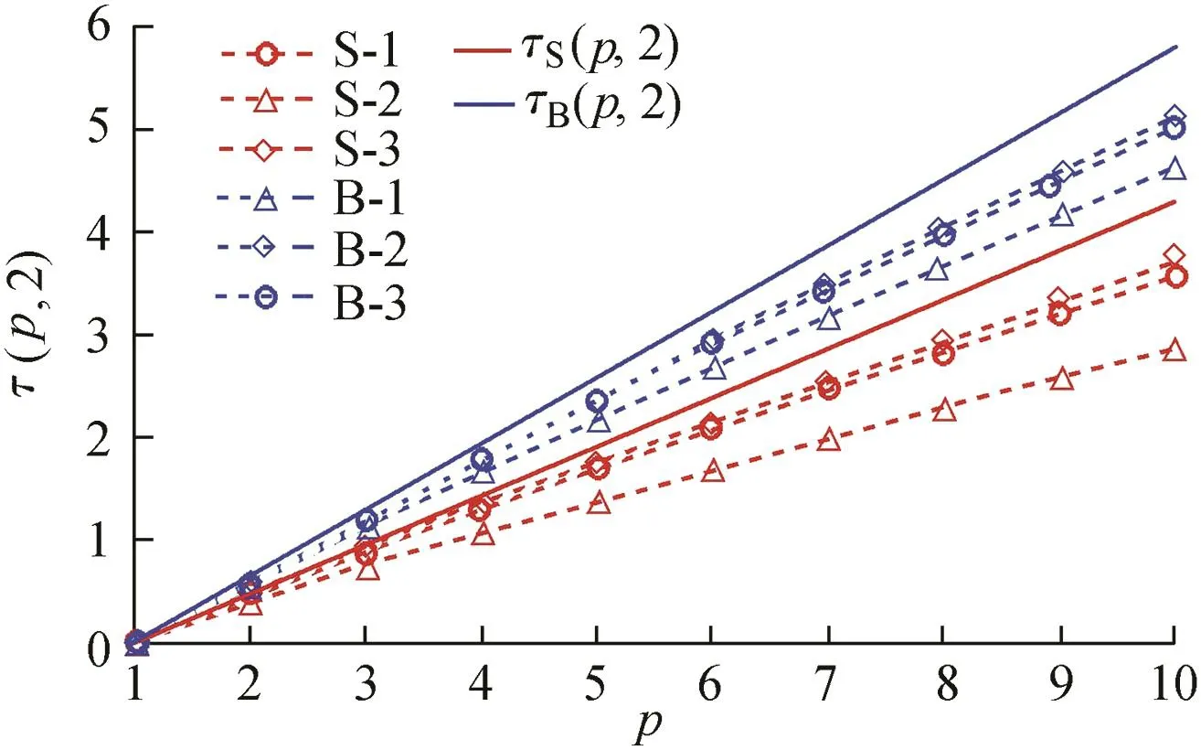
Fig.5.Relationship between ESS scaling index τ（p，2）and order p.

6.Conclusions

In this study,the statistical characteristics of the turbulent flow velocity with a finite Reynolds number in Taihu Lake were analyzed in terms of both the statistical distribution and the reverse structure function.Based on the statistical analysis results,the following three conclusions are drawn:

The velocity PDF presented sharp peaks and heavy tails.This non-Gaussian distribution can be described by the Lévy distribution accurately.Compared with the fitting results of the normal distribution,the Lévy distribution characterizes the tailing information of a power-law heavy-tailed distribution with higher accuracy,and the parametersare reasonable.

The PDF of the reverse structure distance for the velocity in the surface layer can be fitted by the stretched exponential distribution,and shows the independence of velocity difference δu and time.In contrast,the PDF of the reverse structure distance for the velocity in the deep layer has diverse distributions at different scales,and shows dependency on the δu and time.

Using a reverse structure function,the ESS calculation results were obtained.Affected by a finite Reynolds number,the measured turbulent flow velocity has a relative scaling exponent,showing a large degree of deviation between scaling trend estimations in the surface and deep layers.The significant difference indicates that,based on the reverse structure function and the ESS,the turbulent flow velocity is significantly different with different structures.