An Efficient Algorithm for Skyline Queries in Cloud Computing Environments

Zhenhua Huang, Weicheng Xu, Jiujun Cheng, Juan Ni＊

1 School of Computer Science, South China Normal University, Guangzhou 510631, China

2 Department of Computer Science and Technology, Tongji University, Shanghai 201804, China

Abstract: Skyline query processing has recently received a lot of attention in database and data mining communities. However, most existing algorithms consider how to efficiently process skyline queries from base tables.Obviously, when the data size and the number of skyline queries increase, the time cost of skyline queries will increase exponentially,which will seriously influence the query efficiency. Motivated by the above, in this paper,we consider improving the query efficiency via skyline views and propose a cost-based algorithm (abbr. CA) to efficiently select the optimal set of skyline views for storage. The CA algorithm mainly includes two phases:(i) reduce the skyline views selection to the minimum steiner tree problem and obtain the approximate optimal set AOS of skyline views, and (ii) adjust AOS and produce the final optimal set FOS of skyline views based on the simulated annealing. Moreover, in order to improve the extendibility of the CA algorithm,we implement it based on the map/reduce distributed computation model in cloud computing environments. The detailed theoretical analyses and extensive experiments demonstrate that the CA algorithm is both efficient and effective.

Keywords: skyline query; cloud computing;steiner tree; simulated annealing

I. INTRODUCTION

Skyline query processing has attracted much attention recently. It is mainly due to the importance of skyline results in several applications, such as information recommendation,multi-criteria decision making, and intelligent data analysis [1]. Given an input base table BT which totally has k dimensions D={d1,…, dk},a skyline query on the subspace V (V⊆D) returns the objects that are not dominated by any other objects restricted to V. Without loss of generality, we use the “MIN” operation in this paper [2]. It is not difficult to see that there are at most 2k-1 subspace skyline queries can be issued by some user.

Various techniques have been proposed for skyline query processing in database and data mining communities. D. Papadias et al.[3] propose a branch and bound algorithm to progressively output skyline objects on the base table 1ndexed by R-tree. One of the most important properties of this technique is that it guarantees the minimum I/O costs. Z. Huang et al. [4] design a cell-dominance computation algorithm to efficiently obtain skyline objects.Specially, the authors integrate a novel pruning technique into the skyline computation algorithm to dramatically decrease the query cost. D. Pertesis et al. [5] present a scalable and efficient framework for skyline query processing that operates on top of SpatialHadoop,and can be parameterized by individual techniques related to filtering of candidate objects as well as merging of local skyline sets. L.Ding et al. [6] propose an efficient ELM-based two stages query processing optimization model, named ELM to ELM (E2E) model,and then present two query processing executions based on the E2E model. B. Groz et al. [7] present the first algorithms for skyline evaluation in a computation model where the input base table can only be compared through noisy comparisons. X. Han et al. [8] propose a novel skyline join algorithm SEPT on massive data. SEPT utilizes sorted positional index lists with join information which require low space overhead to reduce I/O cost significantly. A. A. Alwan et al. [9] design a model to process skyline queries for incomplete data with the aim of avoiding the issue of cyclic dominance in deriving skylines. M. Nagendra et al. [10] propose two novel skyline-join algorithms, namely skyline-sensitive join (S2J)and symmetric skyline-sensitive join (S3J),to process skyline queries over multiple data sources. Y. C. Chen et al. [11] present a novel modification involving the use of skyline filters to reduce the search space of the skyline query by removing data objects that cannot provide a viable skyline result. S. Liknes et al. [12] propose APSkyline, a new approach for multicore skyline query processing, which adheres to the partition-execute-merge framework. Y. Li et al. [13] design a system model that can support skyline queries in mobile distributed environment and propose an efficient algorithm for processing skyline queries using map/reduce.

We find that existing algorithms mostly focus on the performance of skyline query processing from input base tables. However,skyline computation is CPU-sensitive and I/O-sensitive [14]. Hence, as the data size and the number of skyline queries increase, the time cost of skyline queries will increase exponentially, which will seriously influence the query efficiency.

Motivated by the above fact, in this paper,we change the technical thinking, and consider utilizing the prestoring set of skyline views to reduce the time cost and improve the query efficiency. However, obtaining the exact optimal set EOS of skyline views is NP-hard, which can be proven in Section 3. Hence we propose a cost-based algorithm (abbr. CA) to quickly select the optimal set of skyline views. The CA algorithm first gives the cost evaluation model of skyline computation from a skyline view to another skyline view or a skyline query. And based on the cost evaluation model, the CA algorithm finishes the process of obtaining the exact optimal set through two phases: approximate computation and adjustment. In the phase of approximate computation, the CA algorithm reduces the skyline views selection to the minimum steiner tree problem [15] and obtain the approximate optimal set AOS of skyline views. While in the phase of adjustment,the CA algorithm efficiently adjusts AOS and produce the final optimal set FOS of skyline views based on the simulated annealing [16].We theoretically prove that the CA algorithm has the polynomial time complexity and the lower bound of accuracy of 63%. Moreover,in order to improve the extendibility of the CA algorithm, we implement it based on the map/reduce distributed computation model in cloud computing environments [17, 18]. The detailed theoretical analyses and extensive experiments demonstrate that the CA algorithm is both efficient and effective.

The rest of the paper is organized below:Section 2 gives the problem description of our paper. Section 3 presents the method for exactly obtaining the optimal set of skyline views.In Section 4, we propose the CA algorithm to quickly produce the optimal set of skyline views based on the map/reduce distributed computation model. We present the experimental study in Section 5. Finally, Section 6 concludes the paper with directions for future work.

II. PROBLEM DESCRIPTION

In this section, we give the problem description of obtaining the optimal set of skyline views.

Give a k-dimensional full space D={d1,…,dk}, a set of objects BT={p1,…, pn} is said to be a base table on F if each object pi∈BT is a k-dimensional object on F. We use pi[dx] to denote the x-th dimension value of pi. For each dimension dx, we assume that there exists a total order relationship, denoted by ≺x, on its domain values. Here, ≺xcan be ‘＜’ (i.e., MIN)or ‘＞’ (i.e., MAX) relationship according to the user’s preference [2]. For simplicity, in the following definitions, we assume that each ≺xrepresents ‘＜’.

Definition 1 (Dominance relationship).An object p is said to dominate another object r on the subspace V (V∈F) if it satisfies the following two conditions: (1) ∀dx∈V, p[dx] ≤r[dx]; and (2) ∃dx∈V, p[dx] ＜ r[dx]; For simplicity, we use r≺Vp (r⊀Vp) to denote the relationship that p dominates (does not dominate) r on V. Moreover, we regard the full space F as a special subspace.

Definition 2 (Subspace skyline object).Let BT be the set of k-dimensional objects. An object p is a skyline object in BT on V (V⊆F)if and only if there does not exist any other object r∈BT such that p ≺Vr. We use subS(BT,V) to denote the set of skyline objects in BT on V.

Definition 3 (Subspace skyline query).The subspace skyline query subSQ(BT, V) returns the set of skyline objects in BT on V, i.e.,subS(BT, V).

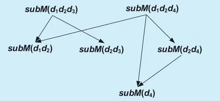
Fig. 1. The skyline view lattice L(N, E).

It is not difficult to see that for a k-dimensional full space, there are at most 2k-1 subspace skyline queries can be issued. For simplicity, we abbreviate subQ(BT, V) by sub-Q(V).

Definition 4 (Subspace skyline view).For a subspace skyline set subS(BT, V), we can materialize it and produce the subspace skyline view subM(BT, V).

Obviously, subS(BT, V)=subM(BT, V). For simplicity, we abbreviate subM(BT, V) by sub-M(V).

Definition 5 (Skyline view lattice).Given an input base table BT which totally has k dimensions D={d1,…, dk}. Then form subspace skyline views subMS={subM(V1),…,subM(Vm), Vi⊆D (1≤i≤m)}, we can organize them as a skyline view lattice L(N, E) which is a directed graph and satisfies the following conditions:

(1) N=subMS={subM(V1),…, subM(Vm),Vi⊆D (1≤i≤m)};

(2) E={＜subM(Vi), subM(Vx)＞|subM(Vi),subM(Vx)∈subMS and Vx⊂Vi}.

It is not difficult to see that if m subspace skyline views are determined, then their corresponding skyline view lattice L(N, E) is also determined and unique.

For example, assume that the input base table BT has four dimensions D={d1, d2, d3,d4} and the system has 6 subspace skyline views subMS={subM(d1d2d3), subM(d1d2d4),subM(d1d2), subM(d2d3), subM(d2d4), sub-M(d2), subM(d4)}. Then we can obtain the skyline view lattice L(N, E): (1) N=subMS;(2) E={＜subM(d1d2d3), subM(d1d2)＞,＜subM(d1d2d3), subM(d2d3)＞, ＜subM(d1d2d4),subM(d1d2)＞, ＜subM(d1d2d4), subM(d2d4)＞,＜subM(d1d2d4), subM(d4)＞, ＜subM(d2d4),subM(d4)＞}. Figure 1 shows the skyline view lattice L(N, E).

Definition 6 (Skyline view-query graph).Given the skyline view lattice L(N, E) and the set of skyline queries SQ={subQ(U1),…,subQ(Un)}, we can construct the skyline view-query graph G(F, G, W) which is a directed weighted graph and satisfies the following conditions:

(1) F=N∪SQ;

(2) G=E∪{＜subM(V), subQ(U)＞| sub-M(V)∈N and subQ(U)∈SQ and U⊂V};

(3) W(＜node1, node2＞∈G)=cost(node1,node2), the computation cost of obtaining node2from node1, which is evaluated in the following part (please see Formulas 1-3 for detail).

For example, given the skyline view lattice L(N, E) in Figure 1 and the set of skyline queries SQ={subQ(d1d3), subQ(d3)}, the skyline view-query graph G(F, G, W) can be shown in Figure 2.

The I/O cost iocnode1can be easily obtained and is expressed below:

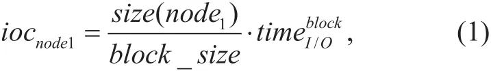
where size(node1) is the size of node1, block_size is the block size, andis the time cost of transferring a block.

We then give the CPU cost cpucnode1→node2as follows (Theorems 1 and 2) [19]. Without loss of generality, we assume that the subpace of node2is U, and let u=|U|.

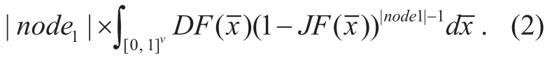
Theorem 1.Let JF(x1,…, xu) denote the joint distribution function of node1on the subspace U, i.e., it denotes the probability[X1≤x1,…, Xu≤xu]. Similarly, let DF(x1,…, xu)denote the join density function. For simplicity, we write (x1,…, xu) as. Then the expect value EC(|node1|, u) of the nmuber of objects in node2can be denoted as:

Theorem 2.Let JF(x1,…, xu) denote the joint distribution function of node1on the subspace U, i.e., it denotes the probability[X1≤x1,…, Xu≤xu]. Similarly, let DF(x1,…, xu)denote the join density function. For simplicity, we write (x1,…, xu) as. Then the CPU cost cpucnode1→node2can be denoted as:

Definition 7 (Feasible solution).Given the skyline view-query graph G(F, G, W) in Definition 6, a feasible solution is a subgraph SG(F’, G’, W’) of G(F, G, W) which satisfies the following conditions:

On the afternoon before Jurgen s departure from home, and beforethe murder, Niels the thief, had met Martin at a beer-house in theneighbourhood of Ringkjobing. A few glasses were drank, not enough to cloud the brain, but enough to loosen Martin s tongue. He began to boast and to say that he had obtained a house and intended to marry, and when Niels asked him where he was going to get the money, he slapped his pocket proudly and said:

(1) F’=subCS∪SQ, where subCS={subM(V1),…, subM(Vs)}⊂subM;

(2) for each node in subCS, it at most has one parent node, and for each node in SQ, it has an unique parent node;

(3) for each pair of nodes node1and node2,if ＜node1, node2＞∈G, then ＜node1, node2＞∈G’,and W’(＜node1, node2＞)=W(＜node1, node2＞).

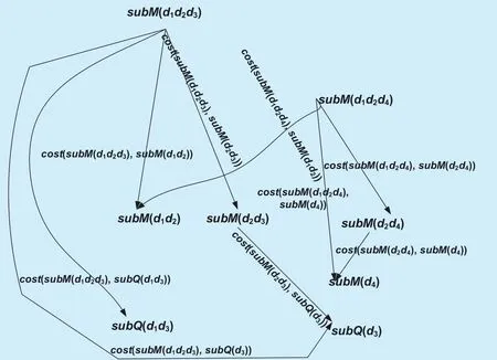
Fig. 2. The skyline view-query graph G(F, G, W).

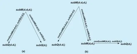
Fig. 3. Two feasible solutions for G(F, G, W).

For example, for the skyline view-query graph G(F, G, W) in Figure 2, Figure 3 shows two feasible solutions.

Problem definition.Given the skyline view-query graph G(F, G, W), for a feasible solution SG(F’, G’, W’) of G(F, G, W), F’includes: (i) s (s＜m) skyline views subCS={subM(V1),…, subM(Vs)}⊂subMS, and (ii)the set of skyline queries SQ={subQ(U1),…,subQ(Un)}. subCS is used to process SQ. And according to our computation cost model (Formulas 1-3), the time cost can be expressed as:scost(SG(F’, G’, W’))=∑∀node1∈F’cost(pnode,pnode1), (4)where pnode is the parent node of node1. In this paper, our goal is to obtain the optimal feasible solution minSG(Fmin, Gmin, Wmin)whose time cost scost(SG(F’, G’, W’)) is minimal and prestore subCSmin∈Fminto process SQ.

III. OBTAINING THE EXACT OPTIMAL SET OF SKYLINE VIEWS

In order to exactly obtain the optimal s skyline views subCSmin, we need traverse the exponential combinations of skyline views in subMS. And it is an NP-hard problem, which can be proved in Theorem 3.

Theorem 3.Givenm subspace skyline views subMS={subM(V1),…, subM(Vm)} and n skyline queries SQ={subQ(U1),…, subQ(Un)},it is an NP-hard problem to obtain and prestore s (w＜m) skyline views subCSmin={sub-M(H1),…, subM(Hs)} from subMS such that scost(SG(F’, G’, W’)) is minimal.

Hence the time complexity O(m,n) of exactly obtaining subCSminequals FS(1)+…+. From O(m,n), we can see that exactly obtaining subCSminneeds exponential time complexity, which belongs to NP Problem. On the other hand, for a given feasible solution FS which includes r skyline views {subM(H1),…, subM(Hr)}⊂ subMS, deciding whether if FS is optimal can be reduce to the minimum cover problem of weighted directed bipartite graph [20]. According to the graph theory [21], we can know that the minimum cover problem of weighted directed bipartite graph is an NP-hard problem. And hence exactly obtaining subCSminis an NP-hard problem.

From Theorem 3, we can see that exactly obtaining optimal s skyline views needs massive CPU and I/O time cost. Hence in the next section, we propose an efficient algorithm CA to fast achieve the approximate optimal solution.

IV. THE CA ALGORITHM

In this section, based on the computation cost model in Section 2, we propose the CA algorithm to quickly obtain the optimal set of skyline views. Detailedly speaking, the CA algorithm mainly includes two phases: (i) approximate computation, and (ii) adjustment.In the first phase, the CA algorithm reduces obtaining the optimal set of skyline views to the minimum steiner tree problem and produce the approximate optimal set subCSappof skyline views (Subsection 4.2). And in the second phase, the CA algorithm adjusts subCSappand efficiently produce the final optimal set of skyline views based on the simulated annealing (Subsection 4.3). Specially, in order to improve the extendibility of the CA algorithm,we implement it based on the map/reduce distributed computation model in cloud computing environments [22, 23] (Subsection 4.1).

4.1 The Distributed Processing Framework of CA

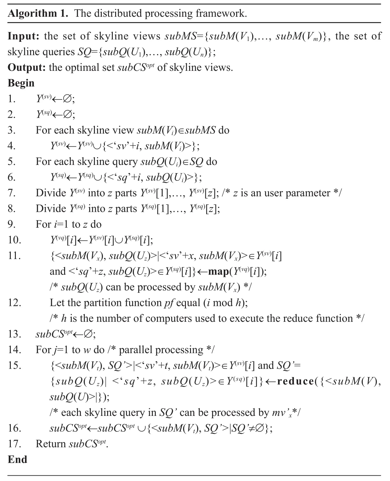
Based on the map/reduce distributed computation model, the distributed processing framework of CA can be shown in Algorithm 1.

In Algorithm 1, under the map/reduce distributed computation model, we first construct two key-value sets Y(sv)and Y(sq)which are related with skyline views and queries respectively. In Y(sv), each pair of key-value consists of a skyline view and its identifier,and in Y(sq), each pair of key-value consists of a skyline query and its identifier (Lines 3-6).Then according to the number z of mappers in distributed networks, the algorithm partitions Y(sv)and Y(sq)into z parts respectively: Y(sv)[1],…, Y(sv)[z], and Y(sq)[1],…, Y(sq)[z] (Lines 7-8). For each Y(sv)[i] and Y(sq)[i] (1≤i≤z), the algorithm calls the map function to realize the efficient optimization the process of obtaining the optimal set of skyline views (Lines 10-11).Moreover, based on the partition function pf,reducers receives the corresponding intermediary key-value set from mappers, and call the reduce function to merges the skyline queries and produces the set SQ’ for the same skyline view subM(Vt) (Line 15). Finally, the algorithm removes those skyline views which are not used to process any query, and returns the remaining ones to users (Lines 16-17).

The map and reduce functions can be shown in Algorihms 2 and 3.

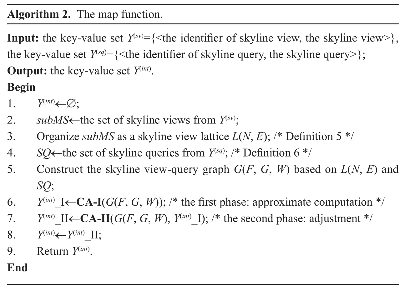
In Algorithm 2, the map funtion first constructs the skyline view-query graph G(F, G,W) based on the input key-value sets Y(sv)and Y(sq)(Lines 2-5). Then the map funtion calls two functions CA-I and CA-II to implement the two-phase optimization. CA-I realizes the first phase, i.e., approximate computation, and CA-II realizes the second phase, i.e., adjustment. The two optimization functions CA-I and CA-II can be implemented in Algorithm 4(Subsection 4.2) and Algorithm 5 (Subsection 4.3).

In Algorithm 3, the reduce funtion takes the key-value set Y(int)as the input parameter and first obtains the set subM S(rf)of skyline views including all skyline views from Y(int)(Line 1).And then the reduce funtion merges the skyline queries and generates the query set SQ[-subM(Vt)] for the same skyline view subM(Vt)(Lines 3-4).

4.2 CA-I: the phase of approximate computation

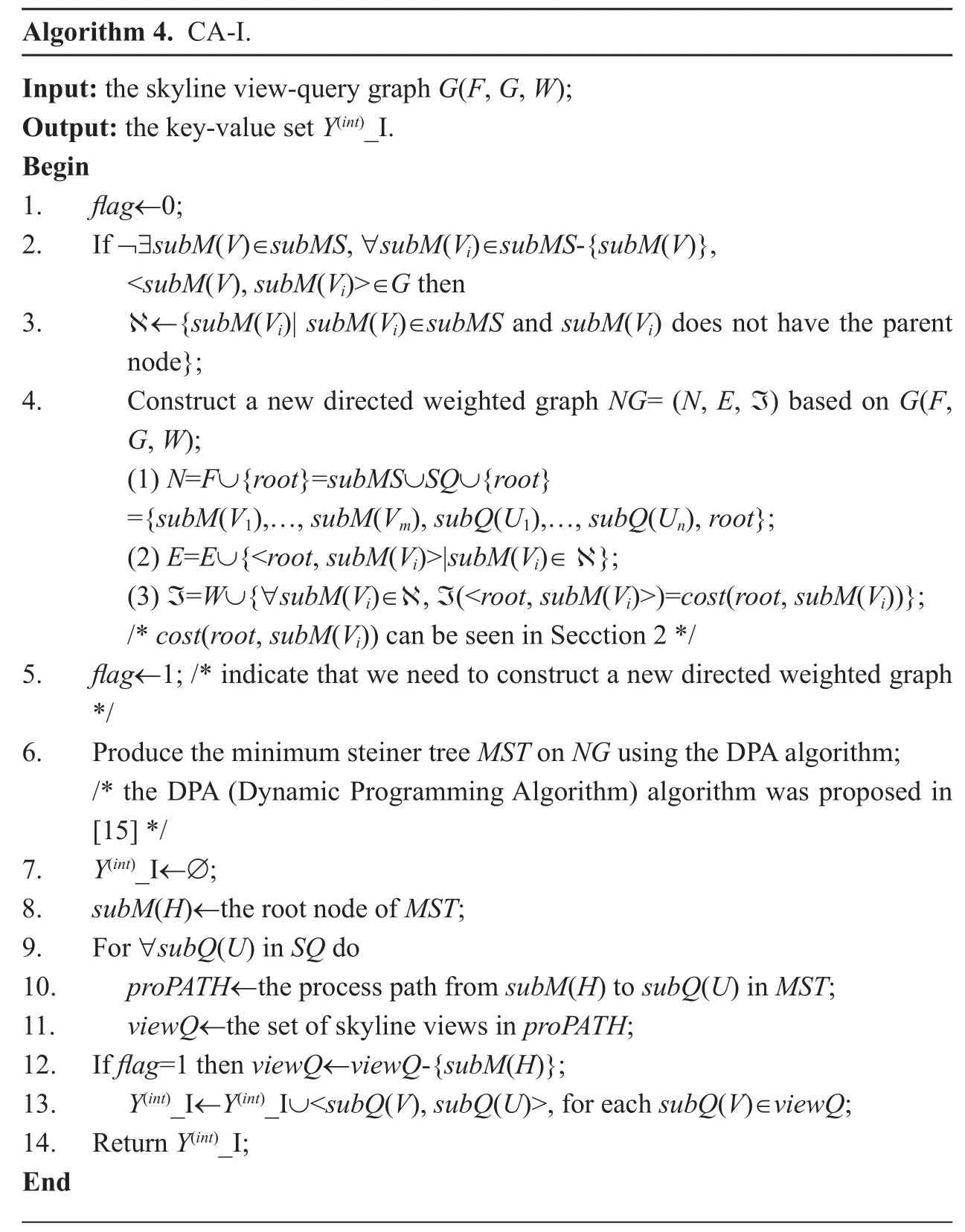
In the phase of approximate computation (CAI), the CA algorithm reduces the process of obtaining the optimal set of skyline views to the minimum steiner tree problem and produce the approximate optimal set subCSappof skyline views. Algorithm 4 shows the implementation process of CA-I.

?

?

?

?

In Algorithm 4, in order to use the DPA algorithm to obtain the minimum steiner tree MST, the CA-I function first checks if there exists a skyline view subM(V)∈subMS such that for each subM(Vi)∈subMS-{subM(V)},V⊃Vi, i.e., ＜subM(V), subM(Vi)＞∈G. If there does not exist such a skyline view, the CA-I function will obtain the set ℵ including the skyline views in subMS which does not have the parent node, and construct a new directed weighted graph NG=(N, E, ℑ) based on G(F,G, W) (Lines 2-4). In NG, the CA-I function adds a virtual root skyline view root which satisfies (let root be subM(H) ): (i) for each subM(V) in subMS, H⊃V, and (ii) there does not exist a skyline view subM(H’) such that subM(H’) satisfies (i) and H⊃H’. Meanwhile,the CA-I function adds the edges from root to each skyline views in ℵ and their corresponding weight values. Then based on NG=(N,E, ℑ), the CA-I function utilizes the DPA algorithm to efficiently produce the minimum steiner tree MST (Line 4). After obtaining MST, for each skyline query subQ(U) in SQ,the CA-I function gets the process path pro-PATH from the root node subM(H) to sub-Q(U) in MST, and produces each key-value pair ＜subQ(V), subQ(U)＞ where subQ(V) is a skyline view in proPATH (Lines 9-13). Note that the CA-I function does not return any one key-value pair involving the virtual root skyline view (Line 12).

It is not difficult to see that the phase of approximate computation (CA-I) has the polynomial time complexity, which is shown in Theorem 4.

Theorem 4.Let the set of skyline views subMS={subM(V1),…, subM(Vm)} and the set of skyline queries SQ ={subQ(U1),…, sub-Q(Un)}, then the time cost of the CA-I function equals:

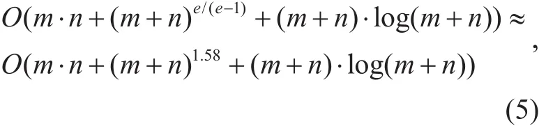
where e is the base of natural logarithm.

Proof.The time cost of CA-I mainly includes three parts:

(1) CA-I needs the time cost O(m) to construct the new directed weighted graph NG=(N, E, ℑ) based on G(F, Γ, W);

(2) CA-I needs the time cost O(m·n+(m+n)e/(e−1)+(m+n)·log(m+n)) to produce the minimum steiner tree MST on G or NG based on the DPA algorithm;

(3) CA-I needs the time cost O(m·n) to produce the set Y(int)_I of key-value pairs.

Hence, Theorem 4 holds.

Below, Theorem 5 theoretically proves that the lower bound of the phase of approximate computation (CA-I) is equal to (e-1)/e»0.63.That is, the query processing cost produced by CA-I is at most e/(e-1)»1.58 of that produced by the exact optimal algorithm which traverses exponential combinations of skyline views.

Theorem 5.Let the set of skyline views subMS={subM(V1),…, subM(Vm)} and the set of skyline queries SQ={subQ(U1),…,subQ(Un)}. We assume that the minimum steiner tree produced by CA-I is MST(F(mst),G(mst), W(mst)), and the optimal feasible solution is minSG(Fmin, Gmin, Wmin). Then we can have:

4.3 CA-II: the phase of adjustment

In the phase of adjustement (CA-II), the CA algorithm adjusts the approximate optimal set of skyline views obtained by CA-I, and efficiently produce the final optimal set of skyline views based on the simulated annealing [16].Algorithm 5 shows the implementation process of CA-II.

In Algorithm 5, we adequately utilize the idea of the simulated annealing [16]. First of all, the CA-II function takes the approximate optimal solution IG(F(ig), Γ(ig), W(ig)) as the initial feasible solution (Line 2). IG(F(ig),Γ(ig), W(ig)) is the corresponding the minimum steiner tree of Y(int)_I produced by the CA-I function. Based on IG(F(ig), Γ(ig), W(ig)) and intKY (the initial value is Y(int)_I), the CA-II function produces intKY’ through two ways:the inner exchange of subMS(ig)(Lines 12-15) and the outer exchange between subMS(ig)and subMS-subMS(ig)(Lines 16-22). Whether replace intKY with intKY’ is determined by the metropolis rule [20] (Lines 25-28).

It is not difficult to see that the CA-II function has the polynomial time complexity,which is shown in Theorem 6.

Theorem 6.Let the set of skyline views subMS={subM(V1),…, subM(Vm)} and the set of skyline queries SQ ={subQ(U1),…, sub-Q(Un)}, then the time cost of the CA-II function equals:

?

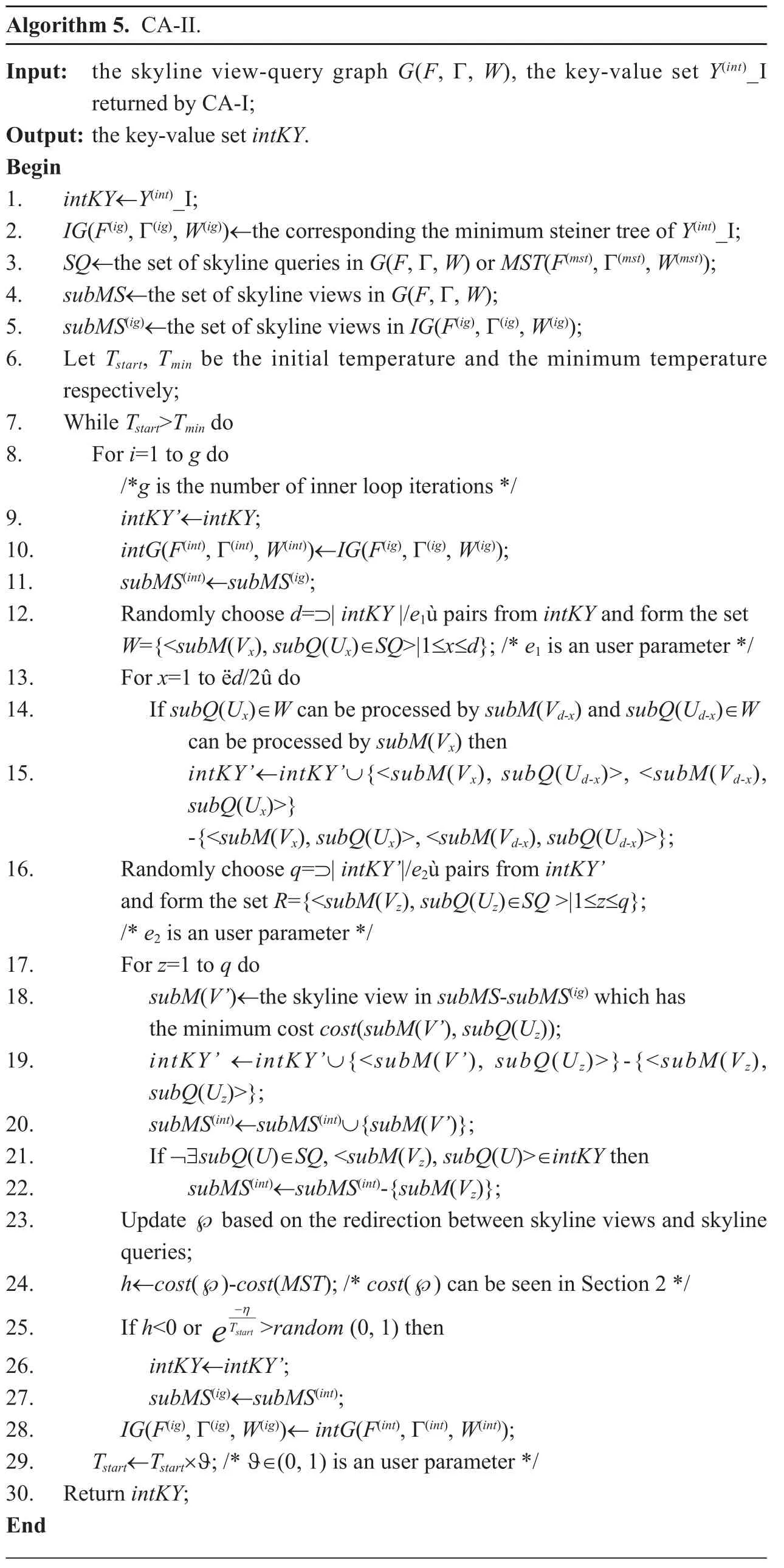
where t and g are the numbers of outer and inner loop iterations (Lines 7 and 8), respectively.

Proof.The time cost of CA-II mainly includes two parts:

(i) O(m·n+m2): the time cost of obtaining the initial feasible solution from the input parameter Y(int)_I;

(ii) O(τ·γ·(m/2+m+m))=O(τ·γ·m ):the time cost of the inner exchange of subMS(ig)and the outer exchange between subMS(ig)and subMS-subMS(ig).

Hence, the time cost of CA-II is O(m·n+m2+τ·γ·m). Thereby, Theorem 6 holds.

V. EXPERIMENTAL EVALUATION

In this section, we experimentally evaluate the optimization accuracy and the time cost of our CA algorithm.

5.1 Experimental Setting

In our experiments, the experimental environment is an Apache Hadoop platform which consists of 40 PC. Each PC has a quad-core i5-3450 CPU, 4G memory, 500G hard drive,and CentOS Linux 6.4 operating system. The version number of our Hadoop platform is 1.0.3.

In the experiments, we produce a 20-dimensional base table which has 5´107objects and 6000 skyline views. And we issue 300 skyline queries.

There are two algorithms compared with our CA algorithm:

(i) OPTIMAL: the algorithm traverses exponential combinations of skyline views to obtain the exact optimal solution;

(ii) GREEDY: for each skyline query sub-Q(U), the algorithm chooses the skyline view which has the minimum cost to process sub-Q(U).

Each class of experiments is divided into two groups:

(i) The number nq of queries is fixed to 300; the number nsv of skyline views varies in the range [1000, 5000];

(ii) The number nsv of skyline views is fixed to 6000, the number nq of queries varies in the range [50, 250].

5.2 Optimization Accuracy Evaluation for The Algorithms

In this subsection, we experimentally evaluate the optimization accuracy of the above three algorithms. Figure 4 shows the results of experiments for these algorithms.

In Figure 4, we take OPTIMAL as the baseline because the set of skyline views obtained by OPTIMAL is exactly optimal. That is, the query processing cost produced by OPTIMAL is least among three compared algorithms.And we let the optimization accuracy of OPTIMAL is equal to 100%.

Fig. 4. Optimization accuracy evaluation for three algorithms.

From Figure 4, we can easily observe that the optimization accuracy of our CA algorithm approaches OPTIMAL’s, while the optimization accuracy of GREEDY is relatively poor.It is mainly because: (i) Our CA algorithm utilizes the minimum steiner tree algorithm(the DPA algorithm [15]) to obtain the approximate optimal solution and uses the simulated annealing to produce the final optimal solution so that the optimization accuracy of the solution can be well guaranteed. (ii) for each skyline query subQ(U), GREEDY chooses the skyline view which has the minimum cost to process subQ(U) and generates the final greedy feasible solution. And this greedy feasible solution is easy to fall into the local optimal problem. For example, in Figure 4(a), when the number of skyline views equals 5000, the optimization accuracy of CA is 96.3% of OPTIMAL’s while the optimization accuracy of GREEDY is only 40.5% of OPTIMAL’s. And in Figure 4 (b), when the number of skyline views equals 5000, the optimization accuracy of CA is 91.9% of OPTIMAL’s while the optimization accuracy of GREEDY is only 39.7% of OPTIMAL’s. Furthermore, we can observe from Figure 4 that: (i) For each experimental setting, the optimization accuracy of CA is not less that 72.6% of OPTIMAL’s,which validates the correctness of Theorem 5 proposed in Section 4. (ii) In Figure 4 (a),the optimization accuracy of GREEDY falls into [38.2%, 55.7%], and In Figure 4 (b), the optimization accuracy of GREEDY falls into[39.7%, 68.2%].

5.3 Runtime evaluation for the algorithms

In this subsection, we experimentally evaluate the runtime of three compared algorithms.Figure 5 shows the results of experiments for these algorithms.

Although the optimization accuracy of OPTIMAL is slightly higher than CA’s, in Figure 5 we can observe that OPTIMAL take enormous time in the experiments. This is mainly because for obtaining the exact optimal solution, OPTIMAL needs to traverses exponential combinations of skyline views, and therefore has an exponential time cost. While CA only needs the polynomial time complexity to return the approximate optimal solution and its runtime is close to the one of GREEDY. For example, in Figure 5 (a), when the number of skyline queries equals 250, the runtime of AAORS is only 1.32% of OPTIMAL’s and the runtime of GREEDY is only 0.40% of OPTIMAL’s. And in Figure 5 (b), when the number of skyline queries equals 250, the runtime of AAORS is only 1.28% of OPTIMAL’s and the runtime of GREEDY is only 0.39% of OPTIMAL’s.

Hence, from the experimental evaluation shown in Figure 4 and Figure 5, we can conclude that our CA algorithm can not only balance the optimization accuracy of feasible solution and the running time, but also has a good scalability.

Fig. 5. Runtime evaluation for three algorithms.

VI. CONCLUSION AND FUTURE WORK

It is very meaningful to research skyline queries in cloud computing environments. In this paper, we analyze the main performance drawbacks of existing works, and propose an efficient algorithm CA to efficiently process skyline queries in cloud computing environments.The CA algorithm does not need to implement skyline queries based on massive base data,and just use prestoring optimal set of skyline views to efficiently answer multiple skyline queries. Our CA algorithm utilizes the map/reduce distributed computation model and can fast produce the optimal set of skyline views through two phases: approximate computation and adjustment. The detailed theoretical analyses and extensive experiments demonstrate that our CA algorithm is both efficient and effective.

Future work will focus on designing more exact cost evaluation model, improving the optimization accuracy of our CA algorithm,and on more experimentation.

ACKNOWLEDGMENTS

This work was supported by the National Natural Science Foundation of China (No.61772366), the Natural Science Foundation of Shanghai (No. 17ZR1445900), and the program of Further Accelerating the Development of Chinese Medicine Three Year Action of Shanghai (2014-2016) ZY3-CCCX-3-6002.