Glacier systems response on climate change by the definite climatic scenario: northeast Russia

Maria D. ANANICHEVA & Roger BARRY

1 Institute of Geography, Russian Academy of Sciences, 119017, Staromonetniy pereulok 29, Moscow, Russia;

2 University of Colorado at Boulder, Boulder, Colorado 80309, USA

Abstract In previous papers, we have presented a method for the assessment of the evolution of mountain glacier systems, in which various climate scenarios were used to study the response of glacier systems to climate change. The aim of this study is to assess the evolution of northeastern Russia glacier systems using output from the A-31 climate scenario, and to compare the responses of the different mountain glacier systems to the scenario. We used temperature and precipitation output from the A-31 scenario to assess future evolution of the glacier systems in the Chukchi and Kolyma highlands (for the projection period of 2011–2030), and the Orulgan, Suntar-Khayata, and Chersky ranges (for the projection period of 2041–2060). The paper provides a brief description of the general method that was used and more details on the data and methods used for each glacier system.Responses of glacier systems were analyzed on the basis of four parameters: mean glacier area, system mean altitudinal range,changes in equilibrium line altitude, and glacier area by the end of the projection period. The relationships between the factors received support an applicability of the A-31 scenario to the study of glacier system evolution.

Keywords projection, scenario, glacier reduction, temperature, precipitation, northeastern Russia

1 Introduction*

Although northeastern Russia has been warming since the second half of the 20th century, it is a region that remains poorly explored. Nevertheless, glacier systems here have been sufficiently studied to be included in the USSR Glacier Inventory (Catalogue of glaciers of the USSR,1970–1982).

The term “glacier system” refers to a set of glaciers united by their common links with the environment, for example,glaciers that are located in the same mountain range or archipelago and subjected to similar atmospheric circulation patterns. The glaciers are related to each other usually via parallel links from atmospheric inputs and topographical features to hydrological outputs and topographical channelizations and demonstrate common spatial patterns of glacier regime and other features (Krenke, 1982).

Since the beginning of the 21st century, we have started to conduct field and remote sensing studies of glacier systems in northeastern Russia (Aðalgeirsdóttir et al.,2017; Ananicheva and Karpachevsky, 2015; Ananicheva et al., 2012, 2010). Northeastern Russia is a huge region with many glaciers in its mountain ranges and highlands. In this study, we use temperature and precipitation output from the A-31 climate scenario recommended by the Central Geophysical Observatory in St. Petersburg (Kattsov and Govorkova, 2013) to assess evolution of the glacier systems in the Chukchi and Kolyma highlands (for the projection period of 2011–2030), and the Orulgan Range, Suntar-Hayata Mountains and Chersky Range (for the projection period of 2041–2060).

The A-31 climate scenario has been derived by averaging the model output of 31 global atmosphere–ocean global circulation models that were included in the Representative Concentration Pathway (RCP) experiments of the Coupled Model Intercomparison Project Phase 5(Moss et al., 2007). In particular, RCP8.5 has the strongest forcing and is used for glacier systems with relatively large glacier area, while the more moderate RCP4.5 is used for systems with small glaciers. Model output from the climate scenario includes mean monthly temperature (in °C) and precipitation (in mm·d−1), and their standard deviations over 12 months (as a measure of inter-model scatter) given for grid cell centers and over a 1°×1° grid.

Multi-model ensemble predictions of changes with respect to the reference period are added to Modern Era Retrospective-Analysis for Research Applications reanalysis temperature data and precipitation climatology to obtain absolute values of temperature and precipitation (Xie and Arkin, 1998). Using the techniques developed by Ananicheva et al. (2010), vertical profiles of mass balance for the present time are constructed using available climate data from the second half of the 20th century. These data include Research Unit Time-Series Version 3.22 (CRU TS3.22), which is a set of high-resolution gridded data of month-by-month variation in climate, and monthly global gridded temperature and precipitation data from the University of Delaware (USA) air temperature and precipitation database, which represent an interpolation of data from weather stations. The aim of this study is to use output from the A-31 climate scenario to make projections about the evolution of different glacier systems in northeastern Russia, and to compare the responses of different glacier systems to the scenario. Glacier data are mainly from the USSR Glacier Inventory (Catalogue of glaciers of the USSR, 1970–1982), and are supplemented with more recent inventories for Chukotka and Kolyma glaciers (Sedov, 1997a, 1997b).

2 Evolution of the glacier systems of the Suntar-Hayata Mountains and Chersky Range

We evaluated the projected changes in the glacier systems of northeastern Siberia. We focused on the glacier systems of the northern and southern massifs of the Suntar-Hayata,which cover 111 and 88 km2, respectively. We also studied the glaciers of the Chersky Range in the main massifs of Erikrit, Buordakh, which lies in the central part of the range,and Terehtyakh, which is in the eastern part of the range; they cover 7, 63, and 28 km2, respectively (Catalogue of glaciers of the USSR, 1970–1982). Figures 1 and 2 show the area and elevation distributions of the glaciers of the Suntar-Khayta and Chersky ranges.

The uncertainty in the USSR Glacier Inventory varies from region to region. The inventory of the Suntar-Khayta and Chersky glaciers is of relatively high quality because it was compiled mostly from field measurements made by Koreisha (1991, 1963).

For projections of the evolution of these glacier systems, we first calculated the difference between the elevation of the highest point of the accumulation area and that of the lowest point in the ablation area for glaciers in each glacier system using data from the USSR Glacier Inventory. The basic hypsographic curves showing glacier area distribution with altitude were constructed at 200-m intervals.

Second, vertical profiles of ablation (A) and accumulation (C) were constructed for each glacier system using data from weather stations in Northeast Siberia. The C and A values for a system at the equilibrium line altitude(HELA) taken from their maps (Ananicheva and Krenke,2008; Krenke, 1982) were used for validation of calculation.

3 Calculation of ablation and accumulation

Northeastern Siberia and Far East glaciers are cold-based,and superimposed ice prevails; a significant fraction of meltwater refreezes and then melts again on the surface. In this case, it is possible to use a regional variant of the“global” empirical formula relating A to summer temperature (Tsum) at HELApresented by Krenke (1982):

where A is ablation in mm, and Tsumis the mean summer(June, July, August) air temperature at HELAin °C. Koreisha(1991) used this formula for the Northeastern Siberia glaciers state assessment, and the reliability of it has been confirmed in calculations for Glacier 31 in the reconstruction of the Suntar-Khayata glaciation during the Holocene optimum (Ananicheva and Davidovich, 2002).

Mean summer air temperature over glacier surface (Tg)is obtained according to:

where Tngis the temperature over the rock surface nearby(Davidovich and Ananicheva, 1996).

Accumulation profiles were constructed by transforming solid precipitation (Psol) with a concentration coefficient (Kc)that depends on the prevailing morphological glacier type in a glacier system (Krenke, 1982).

The Psolcontributions for each month and each year were defined by the Bogdanova method (Bogdanova et al.,2002; Bogdanova, 1976). Monthly Psolcontribution varies from zero in summer months, to 70%–99% in winter, early spring and late autumn, to 10%–20% in late spring and early autumn.

To construct profiles of projected A (Аpr) and C (Сpr) for 2040–2069, we used present A and C and assumed that projected temperature shift at each grid point applies across the entire (real-surface) altitudinal range encompassed by that grid.

Ablation was calculated using formula (1) and projected temperature at 2 m from the surface; temperature lapse rate in the projected period was considered to be the same as that of the baseline period, therefore we used the temperature lapse rates that have been defined empirically by Koreisha (1991). Accumulation for the projected period was calculated assuming that the high-altitude precipitation gradient would be the same as that of the baseline period.

We calculated the ratio of Psolto annual total precipitation in the baseline period. Assuming that this ratio changes little, we computed the value of Psolfor the projection period from the total precipitation (mm·d−1)output of the A-31 scenario. Koreisha (1963) measured precipitation gradients up to 2500 m. These were applied to the projected Psolvalue on the surface to obtain vertical Psolprofiles. Using Kc, we calculated Cprfor all glacier systems up to the period 2040–2069. Figure 3 shows an example of the ablation/accumulation profiles.

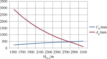
Figure 3 Projected ablation and accumulation profiles for the northern massif of the Suntar-Hayata Mountains.

The value of HELAat the intersection of the Aprand Cprcurves is the mean HELAfor the glacier system in 2040–2069 (HELA-pr). If it shifts to an elevation that is higher than that of the highest point in the accumulation area(Hhigh) of the glacier system, it would mean that the glaciers would disappear under the given climate scenario.

In other cases, it is assumed that the glacier adapts to the new climate in accordance with the Gefer/Kurowski method,and HELAis calculated as the arithmetic mean of the elevations of the highest and the lowest points on the glacier(Kalesnik, 1963). The difference between the elevation of the top of the glacier, Hhigh, and HELA-pris equal to the difference between HELA-prand the elevation of the glacier terminus(Hends). Under the assumption that the same is valid for the whole glacier system, we derive the following formula for the elevation of the lowest point on the glacier:

Changes in HELAand elevation of glacier termini are related via this relationship. Using this simple equation, we obtained the projected elevation distributions of glaciers for 2040–2069. The lowest point on the glaciers coincides with Hends, where glaciated area equals zero, while the highest point on the glaciers remains unchanged. The Gefer/Kurowski method was checked using measured values of HELAfor various glacier systems, and the error was found to be less than 15% (Ananicheva and Krenke, 2008).

The ratio between glacier area change relative to the baseline period and elevation is 0 at Hhighand 1 at Hends. At elevations between Hhighand Hends, the ratio varies between 0 and 1. More details about the method described here are in Ananicheva and Krenke (2007) and Ananicheva et al. (2010).

Table 1 presents results for the projected evolution of northeastern Siberia glacier systems (Suntar-Khayta and Chersky ranges). Detailed description of the techniques and data used for the projections for this region are provided in Ananicheva et al. (2010).

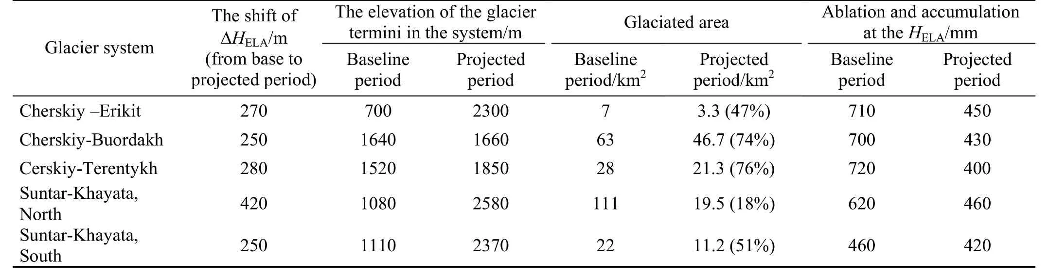
Table 1 Changes of the basic characteristics of the glacier systems in Northeast Asia by the middle of the 21st century(2040–2069)

Table 1 shows that under the A-31 scenario, the glaciers of the northern massif of the Suntar-Hayata are likely to undergo the greatest reduction. This is due to relatively high mean summer temperatures, which are projected to be 14.0°C (area-averaged mean) ±0.5°C(standard deviation). Moderate precipitation of 102±5 mm is also projected. Summer temperature and precipitation of 12.9±0.5°C and 155±5 mm are projected for the southern massif of the Suntar-Khayata. The southern part of the mountains is projected to receive more rainfall due to cyclones from the Sea of Okhotsk. Warming is expected to be more intense in the central part of the northeastern Siberian mountains and basins. Similar results were found in the reconstruction of the state of the Suntar-Hayata glaciers during the Holocene optimum (Davidovich and Ananicheva, 2007), providing validation for the calculation procedure and the chosen climate scenario.

The largest upward shift of HELA(420 m) is projected to take place in the northern massif; upward shifts of HELAin other systems are expected to range from 250 to 280 m.Glacier termini are also projected to shift upward. The largest upward shift of glacier termini (2500 m) is also projected to occur in the northern massif of the Suntar-Hayata, where glacier area is projected to reduce to 18% of that of the baseline period and be only 19.5 km2.Other glacier systems are projected to decrease their area by up to half, as in the case of the Erikrit Massif in the Chersky Range. In the Buordakh and Terehtyah massifs in the central and eastern parts of the Chersky glacier system,projected glacier areas are expected to be 74% and 76% of glacier areas in the baseline period, respectively. Ablation,which is equal to accumulation at HELA, is projected to be maximum in the central part of the Suntar-Hayata(460±10 mm), and minimum in Terehtyah (400±10 mm).Everywhere, ablation is projected to occur at lower elevations than in the baseline period. This is associated with the reduction of glacier area for the projected period.The uncertainty on the calculated value of HELAis 50 m.

Thus, we have shown that applying the chosen multi-model climate scenario of a new generation to mountain conditions, and adopting developed methods to project glacier evolution using the most reliable parameters of current climate produce reasonable estimates. The reliability of this approach has been confirmed by independent assessments of the state of glaciation during the Holocene Optimum.

4 Evolution of Orulgan Range glacier systems

According to the USSR Glacier Inventory, there are mostly cirque and hanging glaciers and only two valley glaciers in the Orulgan Range. The Glacier Inventory contains data on about 74 glaciers covering a total area of 17.38 km2(Catalogue of glaciers of the USSR, 1972). Categorizing the Orulgan glaciers by size, 32.4% of the Orulgan glaciers cover～0.1 km2, 37.8% cover 0.1–0.2 km2, 20.3% cover 0.2–0.5 km2, 4.5% cover 0.5–0.7 km2, 1.4% cover 0.7–0.9 km2, 1.4%cover 0.9–1.5 km2, and 1.4% cover 1.5– 3 km2. The inventory was compiled using aerial photo materials; data error depends upon many factors, the chief of them are: scale of aerial photography, decoding properties of images, image quality. Aerial photographs of 1:50000 and larger scales were used for compiling the inventory of the Orulgan glaciers, and were checked by the authors of the inventory in the field.

The glacier systems consist mainly of cirques(morphological type of corrie) and hanging glaciers.Therefore, we used the moderate scenario RCP 4.5 to assess glacier evolution up to 2041–2060.

For two major glacier systems (Northwest and Southeast of the Orulgan), vertical profiles of A and C were constructed from weather station data using the method described in section 2. Future changes were evaluated relative to the baseline period of 1981–2000. The Orulgan glaciers lie at elevations of 1500 to 2250 m in the north and 1520 to 2280 m in the south (Catalogue of glaciers of the USSR, 1972).For both large glacier systems of the Orulgan Range, values of HELAat the intersection of projected ablation Aprand accumulation Cprcurves were higher than the highest elevation points in the accumulation area. According to the A-31 scenario, HELA-pris projected to be at 2400 m in the northwest and 2460 m in the southeast, implying that the small Orulgan glaciers will not be able to survive under the temperature and precipitation given in the climate scenario.

Table 2 shows that, so far, glacier reduction in the southeast has been larger than that in the northwestern part of Orulgan. Glacier area is now only 56% of that was in time of preparation of the USSR Glacier Inventory, i.e.,approximately 45 years ago. The northwestern part of the region has lost more than 40% of its glacier area(Ananicheva and Karpachevsky, 2015). The equilibrium line altitude has risen by as much as 100 and 70 m in the northwest and southwest, respectively (Table 2).

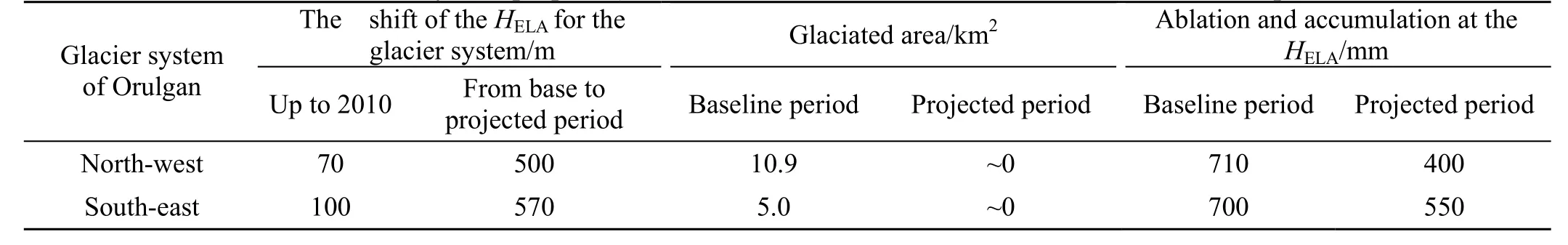
Table 2 Changes of the basic characteristics of the glacier systems in the Orulgan Range between 1967–1968 (when the USSR Glacier Inventory was prepared) and 2010, and in 2040–2069 relative to the baseline period of 1981–2000

Under the A-31 scenario, temperature is projected to increase further in the second half of the 21st century, and projected solid precipitation (Psol-pr) is unlikely to be able to compensate glacier mass loss caused by melting; the glaciers are likely to disappear. Ablation at НELAis projected to drop sharply, and would naturally become zero following the glaciers’ disappearance.

5 Evolution of the Chukchi Highlands glaciers

The Chukotka glacier system comprises small glaciers from 0.1 to 1–2 km2in area. As a result, temperature and precipitation data from the A-31 climate scenario under RCP4.5 were used to predict future changes of the Chukotka glacier system. According to Sedov (2001, 1997a,1997b), glaciers of the Chukchi Highlands are represented by several groups. The first group of three glaciers is located in the northeast of the Chukotka Peninsula in the Teniany Range in the Lavrentiya Bay (Lawrence Bay), and mean HELAis 500 m above sea level. The second group is in the Providence Massif. The HELAof the 14 cirque glaciers ranges from 400 to 550 m. The third group is in Iskaten Ridge near the Cross Gulf of the Bering Sea. The HELAof the 21 glaciers ranges from 500 to 1000 m. The fourth group consists of four glaciers, each of ～0.3 km2in area, and is located on the Pekulnei Ridge. The mean HELAis 740 m.

The fifth group contains five glaciers from 0.1 to 0.5 km2in area with an average HELAof 1400 m. It is situated on Chantalsky Ridge in the Amguema River basin (Sedov,1997a, 1997b). The inventory of the Chukchi glaciers and the Kolyma Highlands is of high quality because it was compiled from measurements made by R. V. Sedov during his field expeditions. The Randolf Glacier Inventory (Cogley,2009) is not included in this dataset. The distribution of glaciers of the Iskaten Range with altitude zones is given in Figure 4.

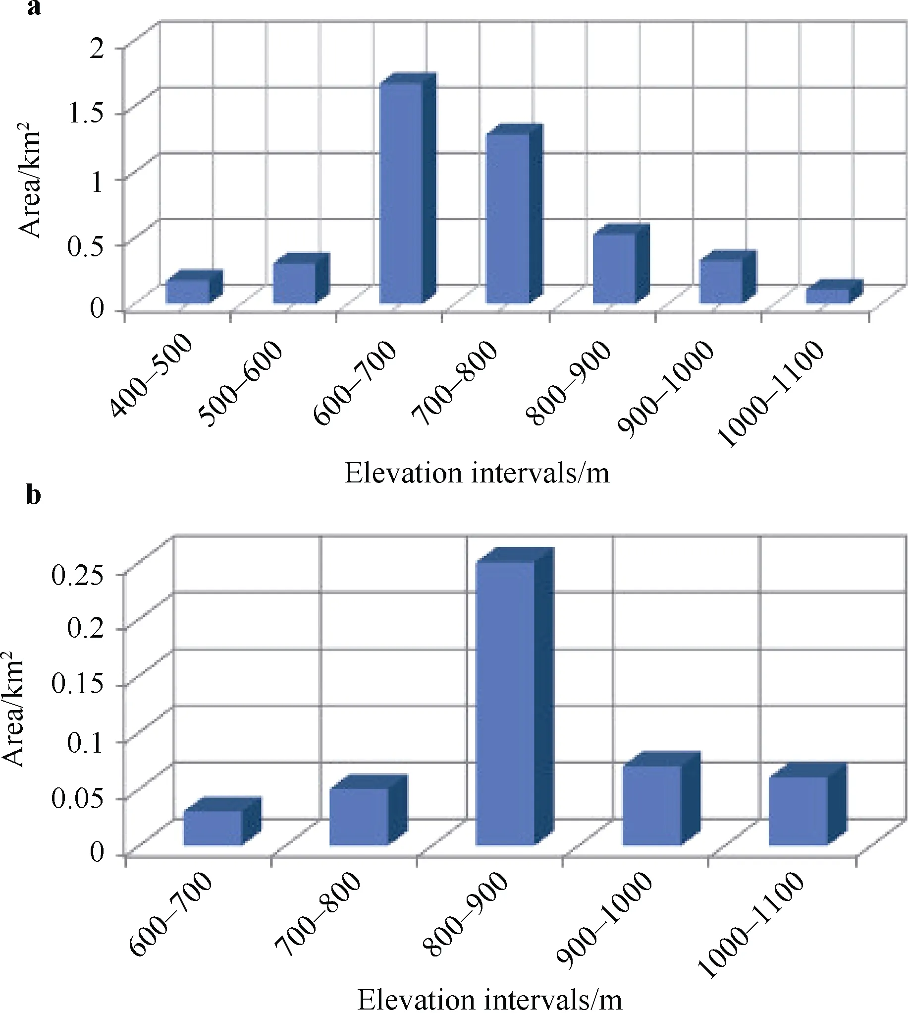
Figure 4 Distribution of ice area by elevation intervals of Iskaten Range glaciers in the Cross Inlet Basin and Sea of Ohotsk(a) , and Chukchi Sea basin (b).

To assess possible variations in the evolution of the Chukotka glaciers, we constructed mass balances for each glacier system using climate scenario output for 2030 and the limited climate data that are available for this region.

To construct mass balance profiles for the baseline period, we used existing climate records, mainly for the middle and late 20th century. The period of coverage differs little from that of the reanalysis data (1960–2000) used to compare with the changes projected by the models over the next dozens of years. Unfortunately, climate data are available only for stations below 400 m above sea level.

Because of the lack of weather stations in the mountains,we used CRU TS3.22 data to construct the upper part of the profiles. This dataset is produced by the Climatic Research Unit at the University of East Anglia and contains month-by-month variations in climate over the period 1901–2013 on a high-resolution (0.5°×0.5°) grid.

For the four glacier systems (Amguema River Basin,glaciers of the Iskaten Range, Pekulnei Range, and Provedence Massif), vertical profiles of Tsumand Psolwere constructed using data from weather stations (for the lower parts of the profiles) and CRU TS3.22 (for the upper parts of the profiles). The geography of the region around these glacier systems is shown on the sketch provided by R.V.Sedov (Figure 5).

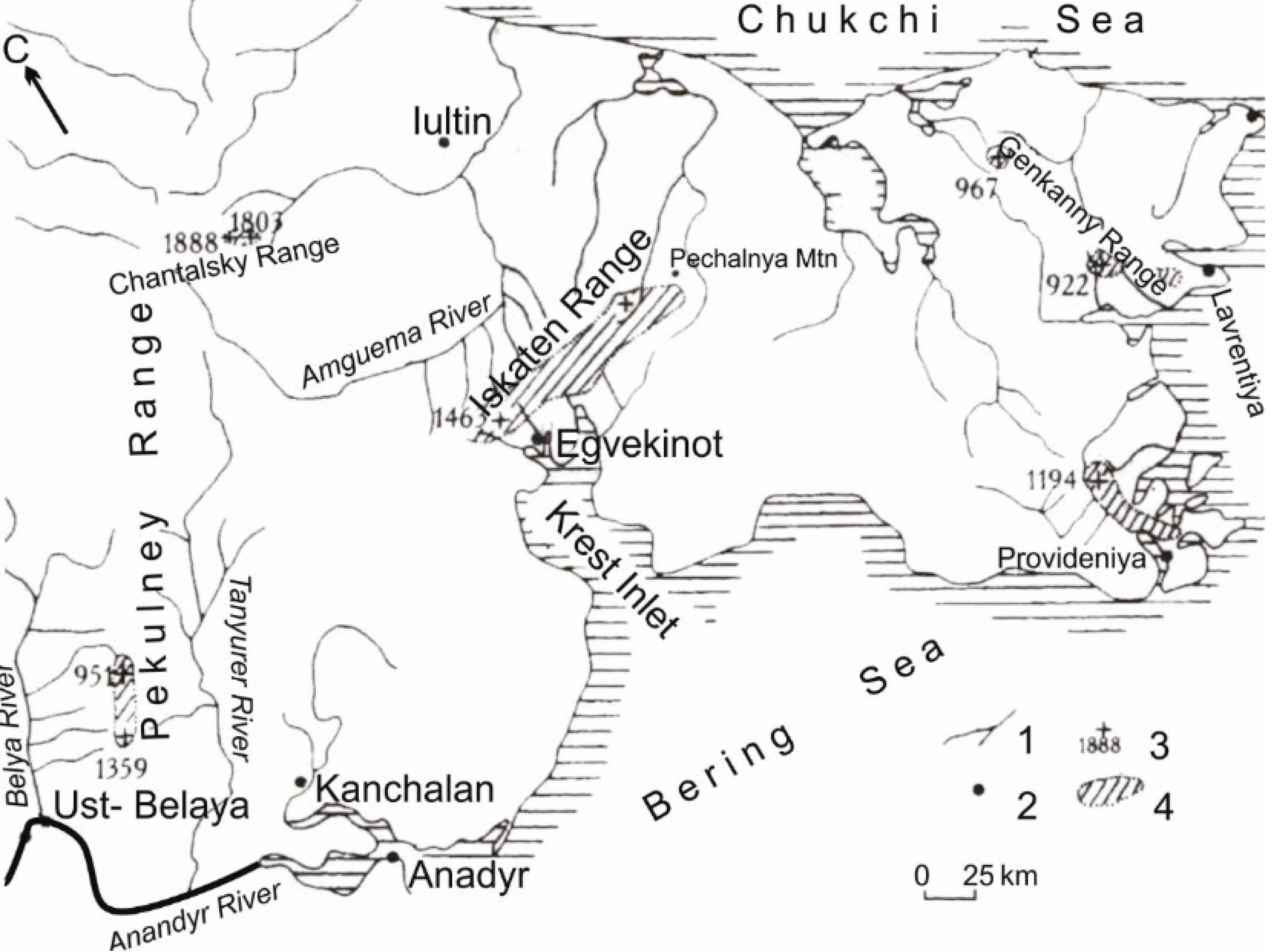
Figure 5 Schematic of Chukchi Highlands with glaciers (courtesy of R. V. Sedov). In the legend, numbers 1, 2, 3, and 4 are next to the symbols for rivers, settlements, spot elevation, and glacierized areas, respectively.

In the Chukchi Highlands, the Iskaten Range and Amguema River basin are areas that are relatively extensively glacierized. To check our assumption whether the precipitation gradients remain unchanged is valid, we calculated precipitation gradients on the basis of climate model output; this procedure was performed on model outputs up to an altitude of ～900 m, which is the maximum altitude at which simulation results are available. The gradients appear to be close to those given by Koreisha(1991) for this mountain range in the 20th century.

Vertical profiles of ablation and accumulation were constructed for the period up to 2030 using Psolid-prand projected mean summer temperature (Тsum-pr) with reference to the average altitude of the glacier system. Projected ablation Aprwas calculated using formula (1). Projected accumulation Cprwas calculated with the help of precipitation gradients from Koreisha (1991). Estimates for the changes in the glaciers of the Chukchi Highlands are presented in Table 3.

Table 3 shows that, under the A-31 scenario, glaciers of the Chukchi Highlands are projected to have reduced in size in different ways by 2030. Small glaciers are projected to disappear completely from Pekulnei Range. By 2030,glacier areas of Iskaten Ridge (Cross Bay) and Providence Bay Massif are projected to be only 6.1% and 13.6% of their values in the baseline period. In addition, НELAis expected to have shifted upward by 300 m by 2030. The glaciers in the Amguema River basin, in northeastern Chukotka are projected to be better preserved with the glacier area projected to be 60% that of the baseline period.However, glaciers in the Amguema River basin are small,and glaciers are projected to cover only ～0.7 km2by 2030.On the basis of the climate scenario and our calculations,approximately 11.5% of the glacier area than was in the baseline period is projected to remain by 2030.

6 Evolution of the Kolyma Highlands glaciers

Glaciers of the Kolyma Highlands consist of two groups.Five glaciers are located on the eastern slope of the Kolyma Highlands near the western shore of the Sea of Okhotsk;their HELAranges from 700 to 1500 m. Fourteen cirque glaciers are located in the northern part of the Taigonos Peninsula; their HELAranges from 700 to 1000 m.

Figures 6a and 6b show the distribution of glaciers with altitude zones based on the altitudes of the highest and lowest points of each glacier defined by R.V. Sedov. The geography of the region around these glacier systems is shown in Figure 6c. It has been estimated that 40.6% of the glaciers are north-facing,7.6% of them face north northwest, 41.0% face northwest,6.4% face west northwest, and 4.4% face northeast, i.e. the Kolyma glaciers mostly face north northwest, where they receive their nourishment in the form of solid precipitation.

Table 3 Changes of the basic characteristics of the Chukchi Highlands glacier systems between 1967–1968 and 2040–2069

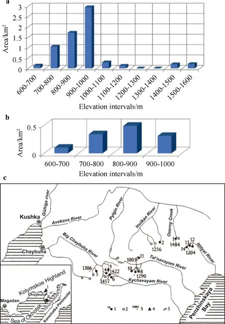
Figure 6 Area distribution of ice by elevation intervals of the Kolyma Highlands. Glaciers of Gizhinginskaya Bay (a), and glaciers of Penzhinkaya Bay (b). Schematic of the Kolyma Highland glaciers (c). In the legend, numbers 1, 2, 3, 4, and 5 are next to the symbols for glaciers and their identification numbers, snow patches, spot elevation, weather stations (I–Gizhiga, II–Taigonos), and glacierized areas, respectively.

We used temperature and precipitation output from the A-31 scenario under RCP4.5 for the period 2011–2030 to predict future changes in the Kolyma Highlands glacier systems.

Climate data from weather stations (precipitation and temperature archive, the University of Delaware database)were used in the construction of vertical profiles of mass balance for Kolyma glacier systems; climate data were used to construct the upper parts of the profiles, while interpolated precipitation and temperature were used to construct the lower parts. To obtain spatial patterns of precipitation of higher resolution we used the Earth topography 5-minute grid,which has a resolution of 1/12°×1/12°. Interpolations from this sparse grid were conducted using a dynamic-statistical method (Ananicheva et al, 2012; Mikhailov, 1986, 1985),which was also used to derive the spatial patterns of solid precipitation in the areas lying between 61.25°N–62.25°N and 155.25°E–162.25°E (Figure 7b). Data from the 0.5°×0.5°gridded global monthly temperature and precipitation data from the University of Delaware, were interpolated on to a grid of 5′×5′ using the following formula:

where t is temperature at elevation h. The dependence of t on h is linear over constant cells for a large net; tmand hmare temperature and elevation at the corners of the grid where elevation is minimum; gradT is the temperature lapse rate as a function t=f(h) (scalar) and is defined empirically (°C·m−1).

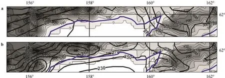
Figure 7 Spatial patterns of solid precipitation over the Kolyma Highlands from the University of Delaware air temperature and precipitation database at a resolution of 0.5°×0.5° (a) , and at a resolution of 5′×5′ (b), interpolated from the University of Delaware data using a dynamic-statistical method.

Vertical profiles of mass balance were constructed for three glacier systems in the Kolyma Highlands on the basis of the relationship of ablation/accumulation with Tsum-prand Psol-pr. The intersection of the ablation Aprand accumulation Cprprofiles indicates the new equilibrium line altitude projected for 2030. Figure 8 shows an example taken from the eastern part of the Taigonos Peninsula.

In the cases where equilibrium line altitude shifts above the elevation of the highest point in the accumulation area of the glacier systems, the corresponding glaciers are likely to disappear under the A-31 climate scenario (Table 4).

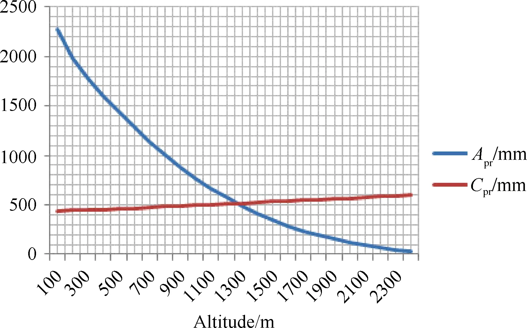
Figure 8 Example of a vertical profile of ablation and accumulation constructed from present climate data. This example is taken from a glacier system in the eastern part of Taigonos Peninsula.

Under the A-31 scenario, HELA-prof the Highlands and Taigonos are likely to exceed 1200 and 1400 m, respectively.These values are the same as the elevations of the highest points in these regions, indicating that the glaciers are likely to be on the brink of disappearance.

7 Comparison of responses of glacier systems under the A-31 climate scenario

Table 5 shows a comparison of the parameterizations of the A-31 climate scenario and projections for the glacier systems included in this study. The Suntar-Khayata Mountains and Chersky and Orulgan ridges are meridional mountain ranges.Therefore, we conducted an analysis of the variation of projected summer temperature (Тsum-scen) and cold period precipitation (Psol-scen) under the A-31 climate scenario with latitude. As latitude increases, Тsum-scenand Psolid-scennaturally decrease. Their maximum and minimum values are indicated in Table 5. Proximity to the ocean is also a factor that influences the magnitudes of Тsum-scenand Psol-scen. These same patterns are characteristic of the Chukchi Highlands glacier systems. The Kolyma Highlands have a quasi-latitudinal orientation;therefore, Тsum-scendecreases as longitude increase, and maximum Psol-scenis found along longitudes next to the ocean.

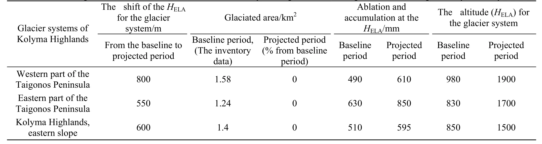
Table 4 Changes of the basic characteristics of the Kolyma Highlands and Taigonos Peninsula glacier systems by 2030

Table 5 Parameterizations of the A-31climate scenario used in this study and model projections for glacier systems in northeastern Russia

To assess the applicability of the A-31 climate scenario to the study of the evolution of glacier systems in northeastern Russia, we analyzed responses of glacier systems to the scenario on the basis of four parameters: mean glacier area (Smean), system mean altitudinal range (ΔH),changes in equilibrium line altitude (ΔHELA), and glacier area by the end of the projected period (Spr). In this study, we have assessed the evolution of different glacier systems using different RCPs and projection periods. Although the data may appear to be heterogeneous, the decision to combine them into one dataset can be justified by the necessity to select specific RCPs and projection periods that would correspond to the sizes and types of glaciers in the various glacier systems.

Figure 9 illustrates the correlations between Smeanand Spr, and between ΔH and Sprfor the glacier systems included in this study. Correlation analyses show fairly close relationships between Smeanand Sprand also between ΔH and Spr; for 14 glacier systems, correlation coefficients between Smeanand Spr, and between ΔH and Sprare 0.73 and 0.84,respectively.

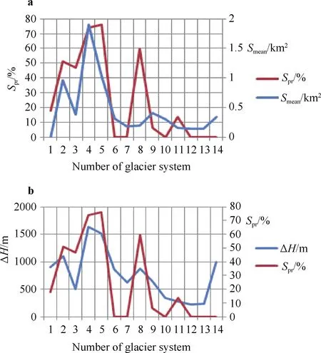
Figure 9 Illustrations of correlation relationships between Smean and Spr (a), and ΔH and Spr (b). Numbers on x-axis correspond to the different glacier systems included in the study. 1:Suntar-Hayata, north; 2: Suntar-Hayata, south; 3: Chersky-Erikrit;4: Chersky-Buordakh; 5: Chersky Terehtyh; 6: Orulgan Range,northwest; 7: Orulgan, southeast; 8: Chukotka, Amguema River basin; 9: Chukotka, Iskaten Range; 10: Chukotka, Pekulney Range;11: Chukotka, Providence Bay; 12: Kolyma Highlands, western part of Taigonos Peninsula; 13: Kolyma, eastern part of the Taigonos Peninsula; 14: Kolyma Highlands, eastern slope.

Figure 9 shows that, under the climate scenario,glacier systems that cover larger areas and latitudinal ranges are likely to have preserved more glacier area by the projected period. However, ΔHELAis different, and has low and moderate negative relationships with Sprand Smean.Thecorrelation coefficients between ΔHELAand Spr, and illustrate the correlation relationships between ΔHELAand Spr, and between ΔHELAand Smean. Changes in HELAare greater in systems with smaller glacier area or fewer glaciers. The correlation relationships between parameters appear logical, and, hence, support the applicability of climate change scenarios to the investigation of glacier systems evolution.

A multiple regression was calculated to predict Sprfrom Smean, ΔH, and ΔHELA. A significant regression equation was found (p = 0.008) with an R of 0.822, and a standard error of the estimate of 19.1. The final predictive model is:

As can be seen in Table 6, Smeanhas a small partial correlation coefficient and a high standard error of correlation coefficient, which exceeds the value of the partial correlation coefficient, indicating that Smeanhas practically no effect on Sprand can be excluded from the prediction model. Conversely, ΔH, and ΔHELAhave larger effects on Sprfor the glacier systems included in this study.between ΔHELAand Sprare −0.65 and −0.50, respectively,pointing to the logical conclusion that glacier systems that can preserve a larger glacier area will also have less change in their equilibrium line altitude. Figures 10a and 10b

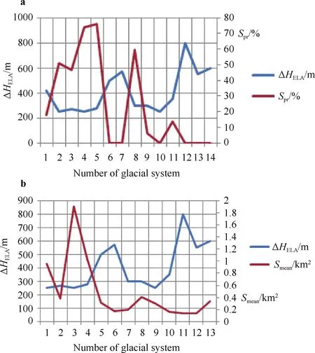
Figure 10 Illustrations of correlation relationships between ΔHELA and Spr (a), and between ΔHELA and Smean (b) . Numbers on x-axis correspond to the different glacier systems included in the study as in Figure 9.

Table 6 Results of a multiple regression to predict glacier area by the end of the projected period (Spr)

It is difficult to conduct a quantitative assessment of the uncertainty in the projected response of glacier systems.Nevertheless, the correlation relationships of the various parameters presented in this section serve as indirect indicators of the uncertainty level, fulfilling a purpose of this study.

8 Conclusions

We have previously developed a method to assess the future evolution of mountain glacier systems using available climate data for the study region. The purpose of this study is to validate the applicability of climate change scenarios to the investigation of the evolution of different glacier systems.

In this study, we applied ONE climate scenario to several regions to test how various glacier systems would respond to the scenario over certain periods in the 21st century. We used the A-31 climate scenario but different RCPs and projection periods. We used temperature and precipitation output from the scenario to assess future evolution of the glacier systems in the Chukchi and Kolyma Highlands (for the period 2011–2030), and the Orulgan,Suntar-Hayata, and Chersky ranges (for the period 2041–2060). Because of the need to study glacier systems of different sizes with numbers of glaciers, it was necessary to apply different RCPs and projection periods to the glacier systems.

Under the A-31 climate scenario, the glacier systems of Suntar-Khayata and Chersky ranges are projected to reduce in extent but not disappear; the small glaciers of Orulgan Range and Chukchi Highlands are unlikely to survive; the glacier systems of Kolyma highland are expected to be on the brink of disappearance.

The response of the glacier systems to the A-31 scenario was analyzed on the basis of four parameters:mean glacier area (Smean), system mean altitudinal range(ΔH), changes in equilibrium line altitude (ΔHELA), and glacier area by the end of the projected period (Spr).Consistency of the results from the analysis is an indirect indication that our assessment of the evolution of the glacier systems was valid.

The relationships between the factors that contribute to the response of glacier systems to climate change validate the applicability of the A-31 climate scenario to the study of glacier system evolution.

AcknowledgmentsI am very grateful to my colleague Alexander Krenke who passed away in 2014. I would like to thank Andrey Mihailov,senior researcher of the Institute of Geography, Russian Academy of Sciences for his help with the calculations. I deeply regret the passing away of my co-author, Roger Barry, distinguished professor and longtime faculty member of the University of Colorado, on 19 March 2018. This work was conducted under the support of the Russian Basic Research Fund(Grant no. N 16-06-00349).