Ill-posedness of Inverse Diffusion Problems by Jacobi’s Theta Transform
2018-08-06FakerBenBelgacemDjalilKatebandVincentRobin
Faker Ben Belgacem,M.Djalil Kateb and Vincent Robin
LaboratoiredeMath´ematiquesAppliqu´eesdeCompiegne,Sorbonne Universit´es,UTC,EA 2222,F-60205 Compiegne,France.
Abstract.The subject is the ill-posedness degree of some inverse problems for the transient heat conduction.We focus on three of them:the completion of missing boundary data,the identification of the trajectory of a pointwise source and the recovery of the initial state.In all of these problems,the observations provide over-specified boundary data,commonly called Cauchy boundary conditions.Notice that the third problem is central for the controllability by a boundary control of the temperature.Presumably,they are all severely ill-posed,a relevant indicator on their instabilities,as formalized by G.Wahba.We revisit these issues under a new light and with different mathematical tools to provide detailed and complete proofs for these results.Jacobi Theta functions,complemented with the Jacobi Imaginary Transform,turn out to be a powerful tool to realize our objectives.In particular,based on the Laptev work[Matematicheskie Zametki 16,741-750(1974)],we provide a new information about the observation of the initial data problem.It is actually exponentially ill-posed.
Key words:Integral operators,regular kernels,Jacobi transform,separated variables approximation.
1 Introduction
In many areas in sciences and engineering,computational methods for the identification of missing boundary data,of pointwise source or of initial states from Cauchy measurements in transient heat transfer seem recurrent(see[1,2,5,8,22]).They are among few pertinent ways to proceed,if not the only ones.The distinctive property of these inverse problems is their ill-posedness;they suffer from serious instabilities(see[3,10,23,26]).Careless numerical procedures used for the approximation of these unstable problems fail most often.We refer to[11]for a general exposition of the possible regularization remedies.The scope here is the ill-posedness degree in the sense of[28]for the reconstruction problems of either the boundary data,the pointwise source or the initial state.In the proofs proposed here,we show how Jacobi Theta functions help to determine how fast the singular values of the underlying operators decreases toward zero,for each of the inverse problems under scrutiny.
The contents of the paper are as follows.Section 2 is a focus on the identification of a missing boundary data,for the diffusion problem.Using Fourier series,we set the inverse problem as a convolution equation;the kernel being an in finite sum of exponentials.Practicing a zoom on this convolution kernel to especially see its shape at the initial time requires a substantial transformation of it.Applying Laplace’s transform to the heat equation,solving it explicitly and using the table of the inverse Laplace transform,we derive a different expansion of that kernel,where the time is inverted in a way.This new expression displays the flatness of the convolution kernel at the initial instant.This statement is enough to ensure the severe ill-posedness or the severe instability of the data completion problem.Section 3 introduces the Jacobi Theta functions and enumerates the identities resulting from the Jacobi Imaginary Transform,resulting itself from Poisson’s summation formula.Thenwe revisit the data completion kernel to show that its transformation can be directly deduced,as a particular example,from the ’inverse’formulas on Jacobi’s Theta functions.In Section 4,we investigate the non-linear problem of pointwise source reconstruction and illustrate that the corresponding linearized inverse problem is severely ill-posed.We turn in Section 5 to the observation problem,currently studied as the adjoint of the exact control of the temperature by a boundary control(see[30]).The novelty the analysis ends to is the exponential ill-posedness of the boundary controllability problem.There is no clues that this statement has been seen before.
2 Boundary data completion
Let a rod be geometrically represented by I,the segment(0,π)of the real axis and J=(0,T)the time interval.We set Q=I×J.The generic point in I is denoted by x and the time variable is t.Assume now be given a boundary condition η in L2(0,T).Then,we consider the following heat equation
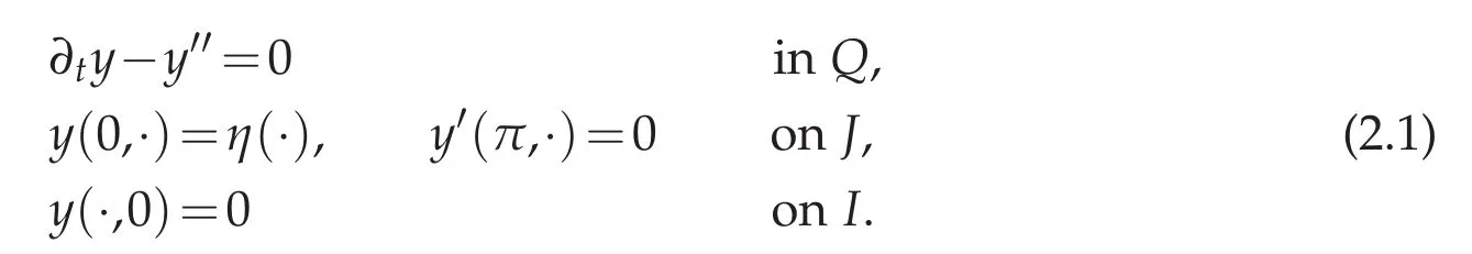
The symbol′is used for the space derivative ∂x.Putting the source data and the initial state to zero is chosen only for simplicity.
The inverse problem of the boundary completion consists in recovering the data η at extremity x=0,which is inaccessible,for some practical reason.Hopefully,it is achieved by collecting observations on y at the other extremity x=π where measurements can be collected.This results in redundant boundary data at point x=π and in unavailable condition at x=0.
Now,consider that h=h(t)is given in L2(J).The boundary condition η(at x=0)is unknown,it is the missing data to be recovered from observation on y at x=π,

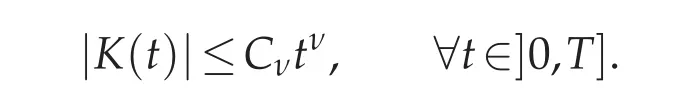
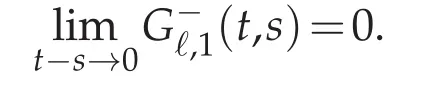
Neumann condition given in(2.1)together with(2.2)are the Cauchy conditions at x=π.The lack of boundary data at x=0 is known to rise high difficulties.The focus here is on the ill-posedness degree.Following the definition in[28],the inverse problem is said to be severely ill-posed if the singular-values(µn)n≥0of the operator D decays faster than any negative power of n.This means that the sequence(nνµn)n≥0decays towards zero for all ν>0.Slightly different definitions may be encountered in the literature;they are all variants of the basic one in[28].We hold the definition we follow here as a pertinent one and is sufficient to our goal.We provide in the subsequent a mathematical proof of the severe ill-posedness of the problem.
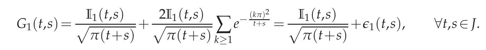
Using Fourier series for the computation of the solution yη,we come up with an integral form
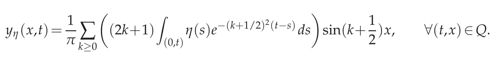
As a result,the observation operator D is as follows
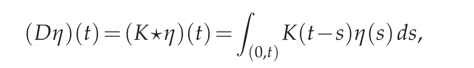
with the kernel K defined to be
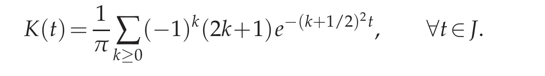
The condensed problem(2.2)turns out to be a Volterra equation and D is a convolution operator with kernel K(·).
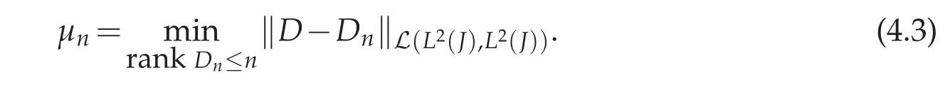
The specialized literature shows that the ill-posedness degree of equation(2.2)is tightly related to the smoothness of the convolution kernel K(·)on J(see[12,27])and in particular to its behavior in the vicinity of t=0.A direct result is that K=K(t,s),looked at a bivariate function,can be approximated,with high accuracy,by a finite sequence of separated functions.This has to do with the concept of Kolmogorov approximation numbers of the operators(see[24]).This is the pursued aim.
Let us first of all notice straight away that,by applying the discrete version of the dominated convergence theorem,K(·)is inde finitely differentiable in]0,T].Hence,the important issue is not only to investigate the differentiability at point t=0+but also to know whether K is flat or not.To get an insight on what happen,we use matlab to depict in Figure 1 the representative curves of K so as of its three first derivatives K′,K′′and K′′.They confirms the expectation.
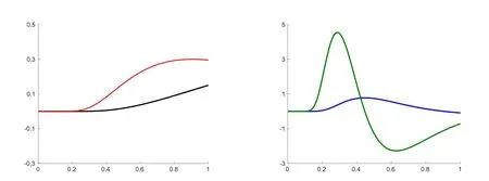
Figure 1:The representative curves of the kernel and its first derivatives,K,K′(left)and K′,K′′(right).They are all flat at the vicinity of zero.
We rigorously show in the sequel that behavior of the kernel K.We therefore need to transform the expression of K.The dominated convergence theorem allows therefore to prove the desired flatness of K to the right of the origin.
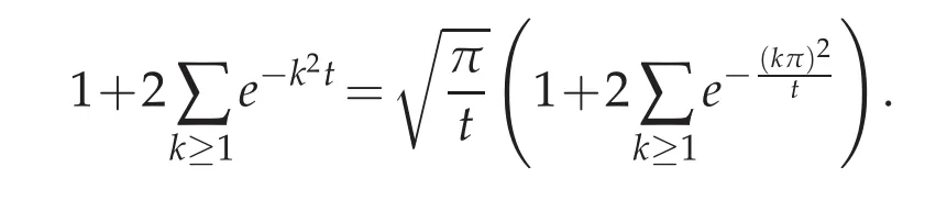
Lemma 2.1.There holds that
Proof.LetLbe the Laplace transform with respect to the time variable.Set=Lyη.Hence,for all p≥0,the functionˆyη(·,p)is solutionof the elliptic boundary value problem
This problem can be explicitly solved.Making all calculations,we obtain that
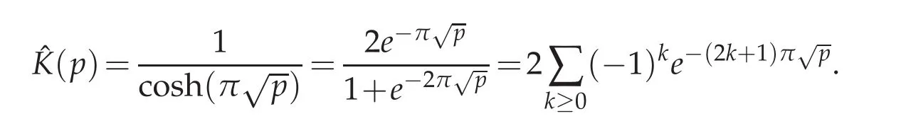
Owing to the convolution theorem of the Laplace transform,we haveThis yields Calling for the table of Laplace transform shows that(see[4,Chapter V,Section 5.6,example 1,page 245]),

This achieves the result and the proof is complete.
Proposition 2.1.For all integer ν,we have that
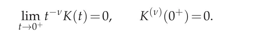
Proof.Using the dominated convergence theorem we are able to check out that for all integer ν,
This is a sufficient indication of the flattened shape of K at the vicinity of t=0.The proof is complete.
A straightforward consequence is that the data completion problem is severely illposed and falls short of exponential ill-posedness.
Corollary 2.1.Problem(2.2)is severely ill-posed.
Proof.Onaccount oftheregularityofK inProposition2.1and following[12],thesingularvalues(µn)n∈Nof the operator D,ordered decreasingly,decay toward zero faster than n−νfor any ν>0.This is the indicator of severe ill-posedness.The proof is complete.
Remark 2.1.Problem(2.2)may not be exponentially ill-posed.K is clearly not analytic near t=0.There is no further indication that the singular-values(µn)n≥0decrease like e−βnνfor some β >0 and ν >0.
3 Jacobi’s Theta transform
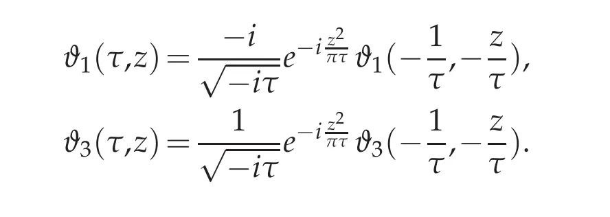
Theta functions enter in a the large category of special functions.Similar to most of special functions,they have an important role in the area of mathematical physics and they enjoy a central utility in the theory of elliptic functions(see[29]).Those we will use thoroughly in our exposition are variants of the fundamental Jacobi theta function introduced in the early 19th century(see[17,1828]).We consider here two of these Jacobi theta functions,depending on two arguments,τ and z,τ and z are complex variables.Both sums are uniformly converging within the domainℑ(τ)>0 and z∈C and these two functions are therefore analytic.Notice that ϑ1and ϑ3are the notations introduced by Jacobi himself for these functions.We do not provide the two remaining functions ϑ2and ϑ4since they won’t be used.
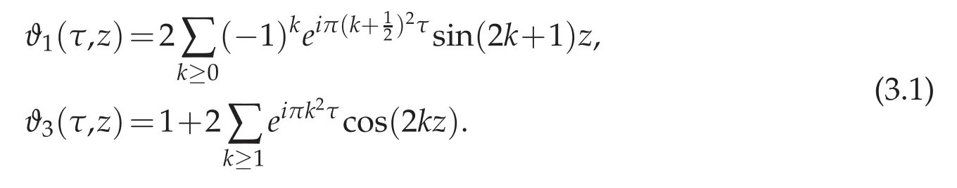
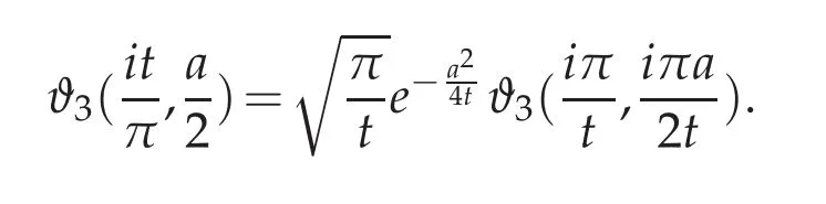
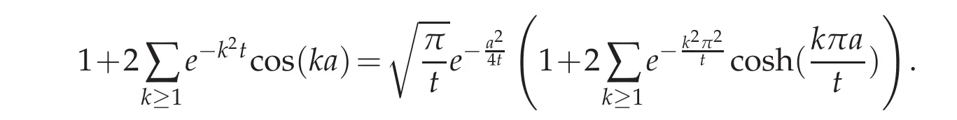
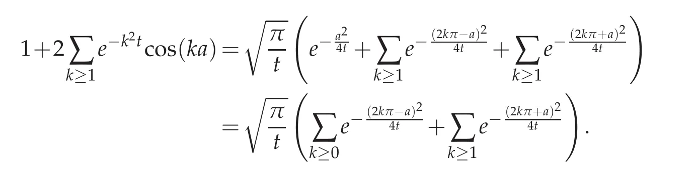
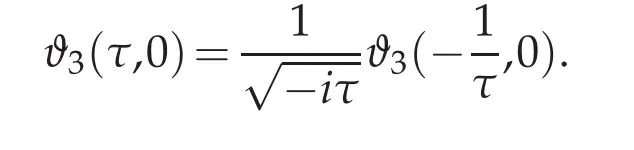
The key result for these functions,we will use repeatedly,is the so-called Jacobi Imaginary transform formula,a fl avor of which has been supplied in Lemma 2.1.The proof is based on the Poisson summation formula and may be found in[29,chapter XXI,page 475].
Lemma 3.1([29]).The following Jacobi identities hold
4 Pointwise source identification
The inverse problem we focus on is the determination of pointwise source from some given observations.It has been addressed in the non-exhaustive list[8,9].The heat equation to work with reads as
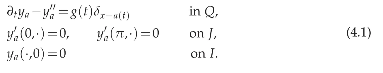
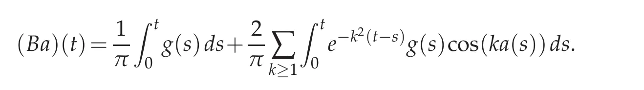
The source g(t)δx−a(t)is eithernot knownat all or only partially knownthat is one among the intensity g(·)or the position a(·)is not available.Consider that a sensor is installed at the extreme point x=0 and that the measurement function h(·)of the temperature y is known.Assume g(·)is known and that the trajectory a(·)of the source does not touch the sensor.This means that a(·)≥a for some constant a∈]0,π[.Then,we are left with the inverse problem: find a(·)satisfying

The operator B is non-linear.Comprehensive identifi ability analysis has been elaborated in[3,16,18].They conclude to the injectivity of B.Despite the fact that ill-posedness degree of non-linear problem,here defined by B,may not be directly linked to its derivative B′(see[25]),we choose to investigate the linearized version of it.Most often,solving(4.2)calls for iterative procedures—Newton,Gradient algorithms.At each iteration,one has to cope with a linearized problem defined by B′.This is why we are rather interested in the linearized operator.
Assume that g∈L2(J)and a∈L∞(J).For a mathematical study of the ill-posedness degree,we calculate a closed form of the solution y using Fourier series.It is given by
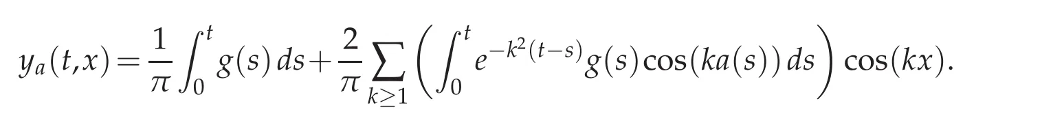
This allows to provide an integral expression of the non-linear operator B which is also the non-linear convolution operator with the kernel
We will know more about the operator B at the vicinity of a∈L∞(J)after studying its Fr´echet derivative D:=B′a.This derivative is expressed as follows:for all f∈L2(J),
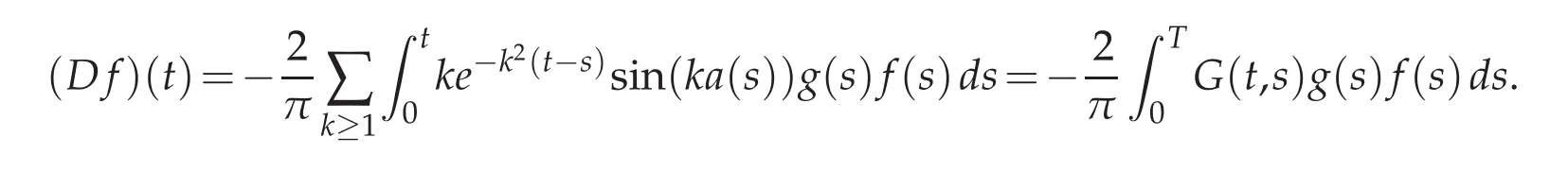
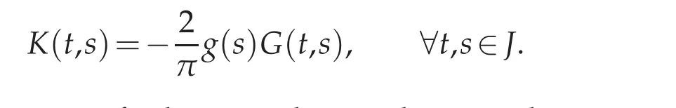
We have set here
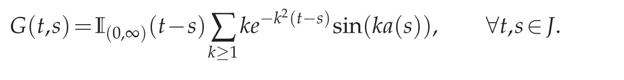
The symbol I(0,∞)is for the indicator function of(0,∞).
Working in a Hilbert framework is better than doing so in Banach spaces.We therefore consider D as an operator mapping L2(J)into itself.We can also study it when it operates from L∞(J)into L2(J).In that context,the spectral theory we have in mind is replaced by the concept of Kolmogorov approximation numbers of the operators(see[24]).
The spectral analysis of D is linked to the smoothness of the full kernel
The hardest part of it consists in finding out the regularity at the vicinity of the diagonal line t−s=0 in the plan(t,s).The Jacobi Imaginary transform is there to help us with this issue.
Proposition 4.1.There holds that:for all(t,a)∈]0,∞[×R.
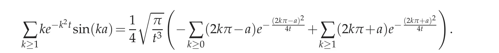
Proof.According to Lemma 3.1,and after settingwe get
Under explicit form,this formula reads as
Replacing cosh in terms of exponentials and reordering yields to
Deriving with respect to a concludes to the desired result.The proof is complete.
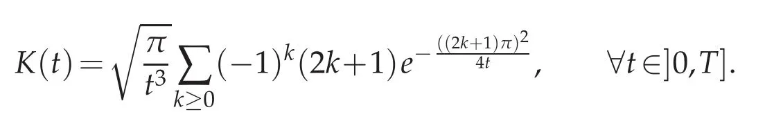
Remark 4.1.Kernels in Proposition 4.1 are plotted in Figure 2 for several trajectories when g=1.If necessary,zooms are realized at the time origin t=0.The flat behavior of these kernels is hence visible either for fixed or moving sources.Notice that the less flat curves are those related to the sources located near the observation point x=0.
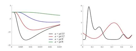
Figure 2:Kernels of Proposition 4.1 for fixed sources at x=a(left).The same kernel for a moving source represented by the black curve(right).The red curve is the trajectory t→a(t).
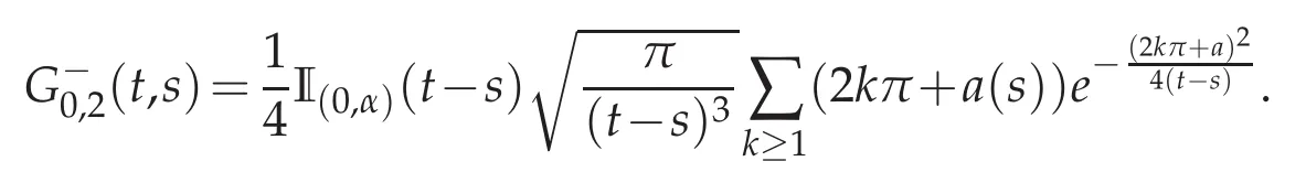
Another preliminary point to deal with is concerned with the regularity of the kernel K,when identifi ed to the following mapping tK(t,·).We begin by studying the(sub)kernel G.
Lemma 4.1.Letℓbe an arbitrary integer.Then,the derivativeG belongs to L∞(J×J).
Proof.The critical point is to clarify the behavior of G near the diagonal line t−s=0.This is the reason why we split the derivativeG as follows

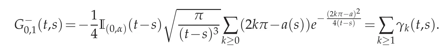
The real number α is positive and small.is supportedaway ofthe diagnonal while the support ofis the narrow strip(of widthembracing the diagonal t−s=0.Each functionandwill be handled in a specific way.We start byThe following statement is straightforward

By the Lebesgue dominated theorem,commuting the derivativeand the in finite sum∑k≥1is authorized.A by-product is that∈L∞(J×J).Addressingrequires the transformation given in Proposition 4.1.It can be expanded as
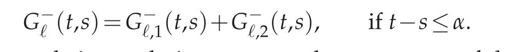
The notations corresponds in an abvious way to the two terms of the expansion of the kernel G.The targeted result is proceeded gradually.
(i)We begin by the derivatives of the( first)in finite sum
Calculate the successive derivatives of the general term γk(·,·)yields
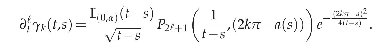
P2ℓ+1is a bivariate polynomial with degree ≤ 2ℓ+1 with respect to each variable.The fact that 0≤a(·)≤π induces the following bound
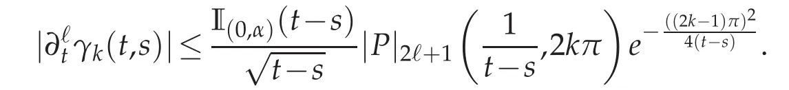
The coefficients of the polynomial|P|2ℓ+1are the absolute values of those of P2ℓ+1.By the dominated convergence theorem,this bound proves not only the uniform convergence of the series(γk)k≥1on the domain 0 ≤ t−s≤ α but also its complete flatness at the diagonal line.Indeed,we have
(ii)The derivatives of the second in finite series
are monitored following the same lines as for the first.This concludes to the same statement that
The proof is then complete.
Toprovidea relevant boundonthesingularvalues ofthe compact operator D we need the following result known as Allahverdiev’s formula(see[14,Theorem 2.1,page 28])
We have the following
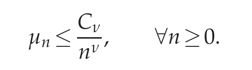
Lemma 4.2.Let ν be a positive real number.There exists Cν>0 for which the singular-values of D satisfy
Proof.The kernel G can be expanded on the Tchebycheff polynomials(Tℓ)ℓ≥0so that

The smoothness of G explains the error estimate(see[15])
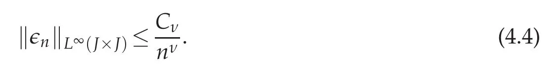
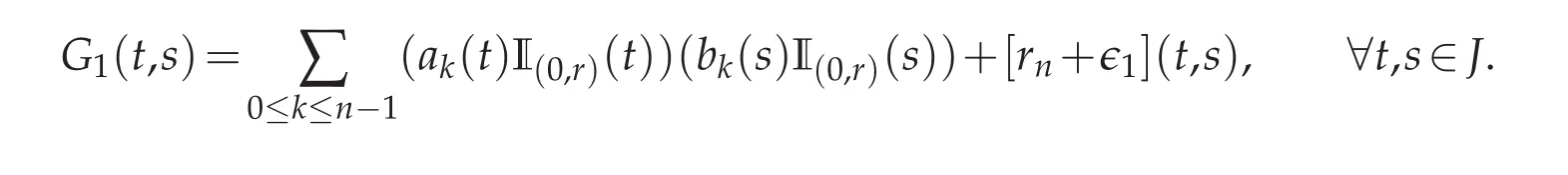
Now,define the kernel Knby
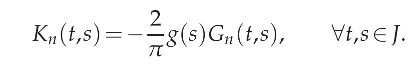
Using(4.4)implies the following bound
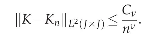
Select Dn,the integral operator with the kernel Kn.It is easily seen that the range of Dnis spanned by(Tℓ)0≤ℓ≤n−1.Its rank is then ≤n.The result is ensued from identity(4.3).The proof is complete
Theorem 4.1.Problem(4.2)is severely ill-posed.
5 Initial state recovery
The third problem we study is concerned with the recovery of the initial state of the heat equation from some observations at the extreme point of the rod.A narrow connection does exist between this problem and the controllability of the heat equation by a Neumann boundary condition.They are adjoint of each other.Here again Theta functions with the Jacobi Imaginary transform turn out to be well-fitting tools for the exploration of ill-posedness degree of both problems.
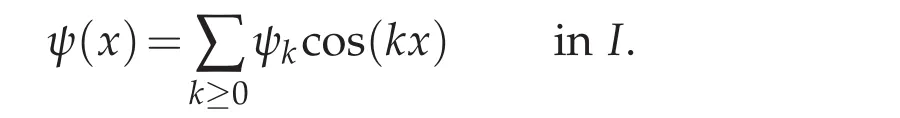
Let be given an initial state ψ∈L2(I).Denote y∈L2(J;H1(I))the unique solution of the boundary value problem
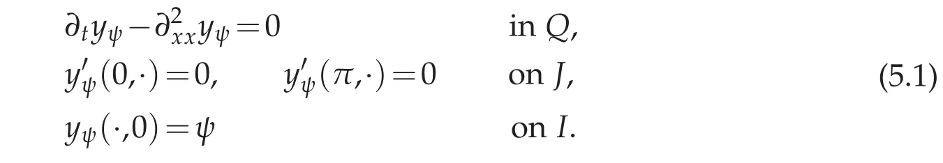
Let h(·)be given in L2(J).The observation equation is expressed as: find ψ ∈ L2(J)such that

This inverse problem is the adjoint of the controllability of the heat equation;the control beingaNeumannconditionat x=0.Ill-posednessresultshave beenprovenforaDirichlet type control in[6].The spectral properties of some in finite structured matrices such as Cauchy and Pick matrices play an important role in the analysis elaborated there.We follow a more direct way to state an improved exponential ill-posedness.
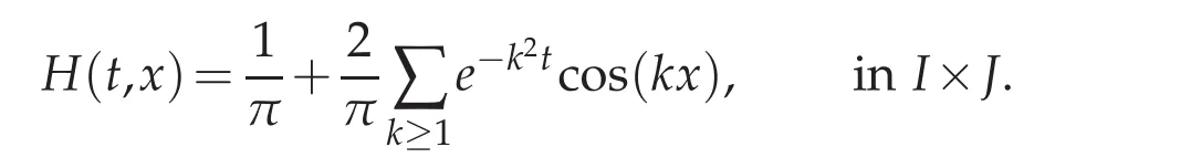
The operator B is bounded from L2(I)in L2(J).We intend to put it in an integral form and to study its kernel.The explicit expression of B comes from Fourier series(see[13,22]).Given that the sequence(cos(kx))k≥1is an orthogonal basis in L2(I),we may expand ψ as
Substituteit into problem(5.1)and after achieving necessary computations,B may be put presented as follows,
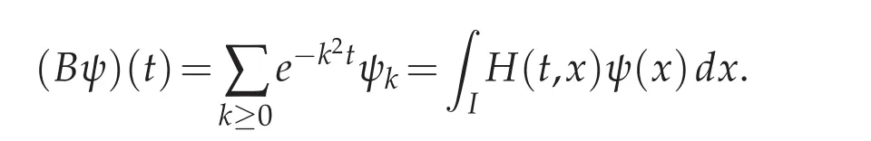
The kernel of the integral operator is hence defined by
Inversion of B amounts to solving the Cauchy sideways problem.This inverse problem has at most one solution(see[19]).Then B is into and its kernelis the trivial subspace,i.e.,N(B)={0}.This tells that the singular-values(µn)n≥0of B are all positive.Investigating the singular-values of B can therefore be carried out by studying the non-vanishing eigenvalues(λn)n≥0of the operator A=BB∗which is also an integral operator
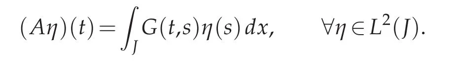
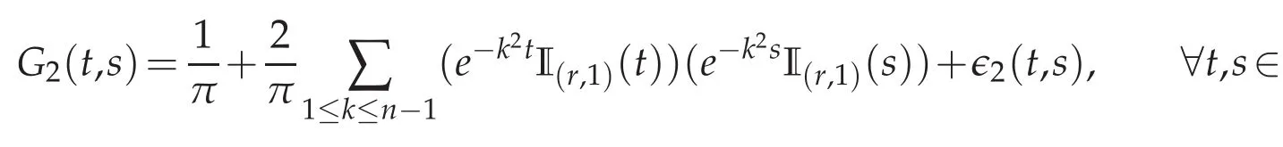
The kernel function G of A is given by

Easy calculations ascertain that G belongs to L2(J×J)and A is in the class of Hilbert-Schmidt operators.Asymptotics of(the singular-values of B)are conditioned by the smoothness of G.Actually G is inde finitely smooth away form the origin(t,s)=(0,0).The key is the behavior of G at the vicinity of the vertex(0,0).We proceed in the sequel to shed some light on this issue.Jacobi’s Theta functions are capable of supplying us with the answer and to lift uncertainty about the behavior of G at the origin.
Lemma 5.1.We have that:for all t,s∈(0,T),
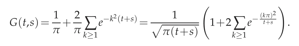
Proof.The Jacobi Theta Transformation on ϑ3,provides
The proof is complete.
The purpose is now to obtain asymptotics of the eigenvalues of the operator A=B∗B.The core questionis therefore the in fluence of the term(t+s)−1/2,in the expressionof the kernel G.Notice that G has a form close to a class of integral operators examined in the early 70’s by A.A.Laptev in[20].A modern approach appears in[7,2006]that simplifies and extendthoseresults to the Banach spaces where the concept of Kolmogorov numbers is used.Recall that Kolmogorov numbers and the singular-values of a linear operator are equivalent in Hilbert scales(see[24]).We will follow this methodology.First of all,we need an important result about the separated expansion of the kernel(t+s)−1/2,
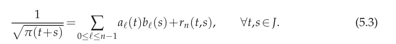
The sequences(aℓ)0≤ℓ≤n,(bℓ)0≤ℓ≤n−1belong both to L2(J).The error estimate we give here can be found in[7].
Lemma 5.2.There exist a sequence(aℓ(t),bℓ(s))0≤ℓ≤n−1such that(5.3)holds with the following error estimation

The constants(C,)are independent upon n.
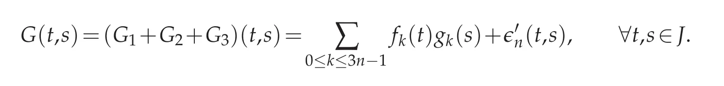
Theorem 5.1.There exist(fℓ(t),gℓ(s))0≤ℓ≤n−1⊂L2(J)×L2(J)such that
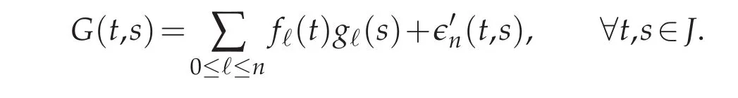
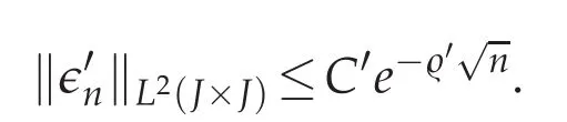
The following estimate holds
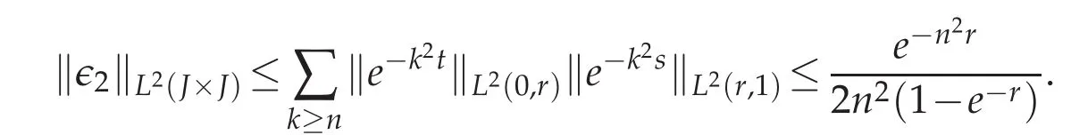
Proof.Let r∈J be a small real number to be fixed later on.Consider the partition of unity
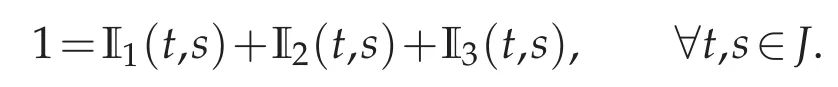
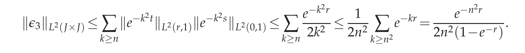
The function I1is the indicator of the small square[0,r]×[0,r],I2is the characteristic function of the strip[0,r]×[r,1]and I3is finally for the strip[r,1]×[0,1].Basically,the proof is obtained after expanding each of the three functions Gi=GIi,1≤i≤3.(i)For the expansion of G3,it is easy to see that

Bounding ∈3(·,·)in L2(J×J)is conducted in a progressive way
(ii)The decomposition of G2is realized following the same lines as above.In fact,we write that J.
with the estimate on∈2,
(iii)The last expansion is for G1.Keeping the exponential family(e−k2t)k≥0in the expression of G1fails to provide an interesting error bound.We hence call for Lemma 5.2 to tansform it,
Plugging expansion(5.3)into the above identity produces the following formula
Estimate for rn(·,·)is predicted in Lemma 5.2.It remains to bound ∈1(·,·)with respect to the norm of L2(J×J).It is derived as follows
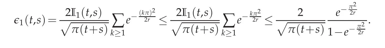
If we switch to the L2-norm then we obtain
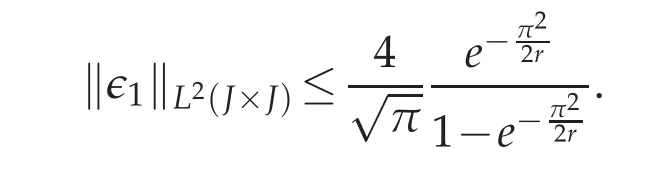
This achieves the third step.
Putting together different expansions of G1,G2and G3,and after re-ordering we derive that
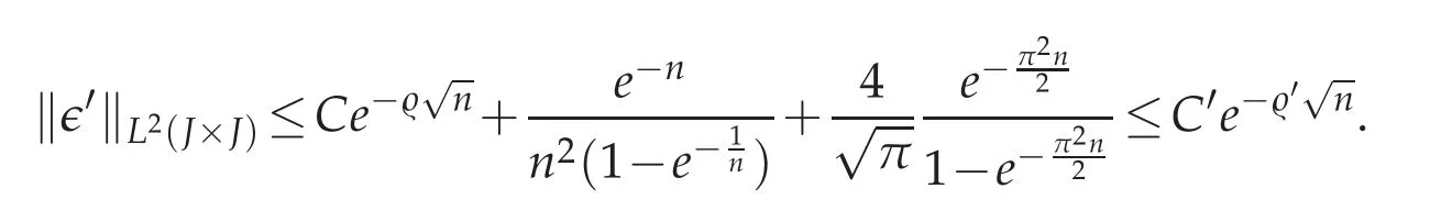
To get the bound on the residual function(·,·),we observe that
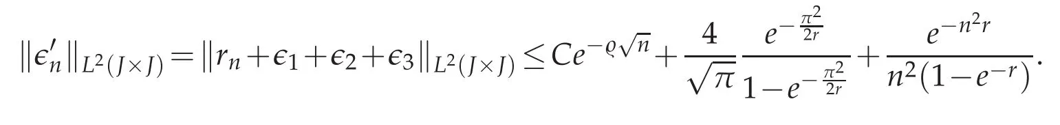
The constant C is of course insensitive to r.Ultimately,selecting r so that r=1/n leads to the final majoration
The proof is complete.
Reproducing the same argumentation as for the former inverse problem of pointwise source detection we derive an exponential decreasing rate of the singularvalues of B.
Corollary 5.1.The singularvalues(µn)n≥0of the operator B decrease like e−′n.The observation problem(5.2)is exponentially ill posed.
Remark 5.1.Investigatingtheill-posednessdegreeofthecontrollability problemby Neumann or Dirichlet boundary data has been addressed in some works(see[13,22,23]).The most advanced results we know of are found in[6].It is shownthere that the singularvalues(µn)n≥0decrease faster than any negative power n−ν,ν>0.The analysis conducted here concludes to additional informations on the decreasing rate of(µn)n≥0.
6 Conclusion
The methdology developed is handy and seems successful for analyzing the compactness of some integral operators,constructed by kernels generated from the heat equation.Jacobi Theta functions and their Imaginary transforms turn out to be strongly fitted to help clarifying some inverse and control questions linked to the diffusion boundary value problems.Hopefully,the mathematical arguments exposed through this paper will be re-insvested for dispersion coupled problem as one can find in[18]and references therein.They might serve to solve further issues related to the diffusion problems.We think in particular of the sensitive question of the exact determination of the control cost††The cost blows up like e/T;computing exactly is interesting for some application,as indicted in[21].for shortime null-controllability of the heat equation.Volterra integral equations with kernels defined by elliptic functions similar to Jacobi Theta functions may also be concerned.
杂志排行

Journal of Mathematical Study的其它文章
- Chebyshev Spectral Method for Volterra Integral Equation with Multiple Delays
- A Diagonalized Legendre Rational Spectral Method for Problems on the Whole Line
- Generalized Hermite Spectral Method for Nonlinear Fokker-Planck Equations on the Whole Line
- POD Applied to Numerical Study of Unsteady Flow Inside Lid-driven Cavity
- Highly Efficient and Accurate Spectral Approximation of the Angular Mathieu Equation for any Parameter Values q