Impacts of Anthropogenic Forcings and El Niño on Chinese Extreme Temperatures

N.FREYCHET,S.SPARROW,S.F.B.TETT,M.J.MINETER,G.C.HEGERL,and D.C.H.WALLOM

1 School of Geosciences,University of Edinburgh,Crew Building,The King’s Buildings,Edinburgh EH9 3FF,UK

2 Oxford e-Research Centre,University of Oxford,Oxford,OX1 2JD,United Kingdom

1.Introduction

Change in the risk of extreme temperatures over China has been a major focus of research(e.g.,Ren et al.,2016;Zhou and Wang,2016;Chen and Zhai,2017;Freychet et al.,2017;Luo and Lau,2017).The impact of anthropogenic forcings has been identified in several studies(e.g.,Sun et al.,2016;Yin et al.,2016,2017;Ma et al.,2017;Peng et al.,2017;Sun et al.,2017)showing an increase in the risk of high temperatures due to an increase in greenhouse gases.Meanwhile,aerosol emissions are understood to have reduced this risk due to their cooling effect(e.g.,Li et al.,2016;Mascioli et al.,2016;Dong et al.,2017),albeit these results are still largely model-dependent(Kasoar et al.,2016).Natural variability also affects extreme temperatures.More specifically,the impact of the El Niño–Southern Oscillation(ENSO)has been documented in several studies and is the leading mode of the interannual natural variability(McPhaden et al.,2016).However,due to the limited period of observations and the low frequency of these events(about two per decade),it is difficult to conduct strong statistical analyses on their impact,especially when investigating the most extreme temperatures.Moreover,ENSO usually exhibits a stronger signal on sea surface temperatures(SSTs)during winter,so most studies have focused on its impact at that time of the year.The influence of ENSO during summer remains difficult to evaluate,although Hu et al.(2013)showed a strengthening relationship between ENSO and extreme temperatures over China during recent decades.

This study uses ensembles with several thousand members to evaluate the risk of summer extreme maximum temperatures over central and eastern China under different conditions.The main objective is to quantify how the most extreme temperatures(during summer)over China are sensitive to different forcings.It is important to evaluate the relative magnitudes of natural variability and anthropogenic influences.Such a study is not easy to conduct with observations only,as ENSO events are limited(about one significant El Niño event every five years)and annual extreme temperatures are rare too.This study aims to contribute to a better understanding of the impact of natural and human drivers of Chinese extreme temperatures,and to provide a statistical approach as a complement to observational-only studies.

Extreme event attribution studies commonly compare ensembles of simulations;particularly,to estimate the impact of greenhouse gases and aerosols relative to a counter-factual natural world[e.g.,Black and Karoly,2016;Sarojini et al.,2016;Zhang et al.,2016;Qian et al.,2018(for recent works);Otto,2017(for a review on attribution techniques)].This method has not been commonly used to investigate how ENSO impacts the risk of extreme temperatures.Black and Karoly(2016)used such a method to analyze Australian temperatures,butfailed to find a clear ENSO signal.In this study,the relative importance of anthropogenic influences(through greenhouse gases and aerosol emissions)is compared to natural variability(i.e.,the role of ENSO,using the 2015/16 El Niño SST signal)using large ensemble simulations.The extended summer maxima of both daily maximum and minimum temperatures are considered.The former corresponds to the most extreme temperature during the day;the latter indicates how warm a night can be and is important for human health as it can lead to exhaustion(Sarofim et al.,2016).

The data and methods are described in section 2 and the results are presented in section 3.Section 4 provides some discussion and concluding remarks.

2.Methods

2.1.Model experiment design

The simulations were run as part of the“climate prediction.net weather@home”distributed computing project,where members of the public donate idle time on their computers to running model simulations.The weather@home setup consists of the Met Office Hadley Centre Atmospheric model(including a land/surface component),HadAM3P,running globally at a horizontal resolution of 1.25◦(lat)×1.875◦(lon).This is one-way-coupled with the Met Office Hadley Centre Regional Model,HadRM3P,running at a resolution of 50 km over East Asia(15◦S–55◦N,70◦–170◦E;Fig.1a).Both models have 19 vertical levels.The models include a sulfur cycle(Jones et al.,2001)and use the Moses 2 land surface scheme(Essery and Clark,2003).The weather@home 2 modeling system is described in detail in Guillod et al.(2017)and hasbeen used previously to study extreme events in many different regions of the world(e.g.,Li et al.,2015;Mar thews et al.,2015;Black et al.,2016;Haustein et al.,2016;Mitchell et al.,2016;Schaller et al.,2016).

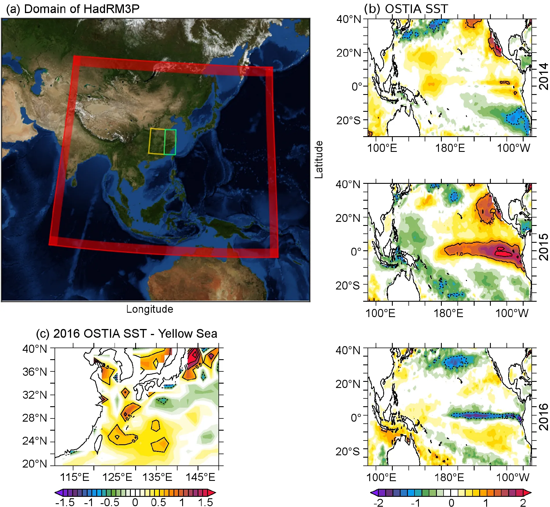
Fig.1.(a)weather@home East Asia 50 km region boundary(red).The shaded area represents the sponge layer in the regional model.The yellow part is the central China region and the green the East China region,used in the returnperiod analysis.(b)OSTIA(Donlon et al.,2012)May–September anomalies of SST(◦C)for three different years,relative to the 1971–2000 summer climatology.For each year,the long-term change has been removed by subtracting the difference(year minus climatology)in the tropical band(30◦S–30◦N)averaged SST.(c)OSTIA 2016 anomalies for the Yellow Sea area only.

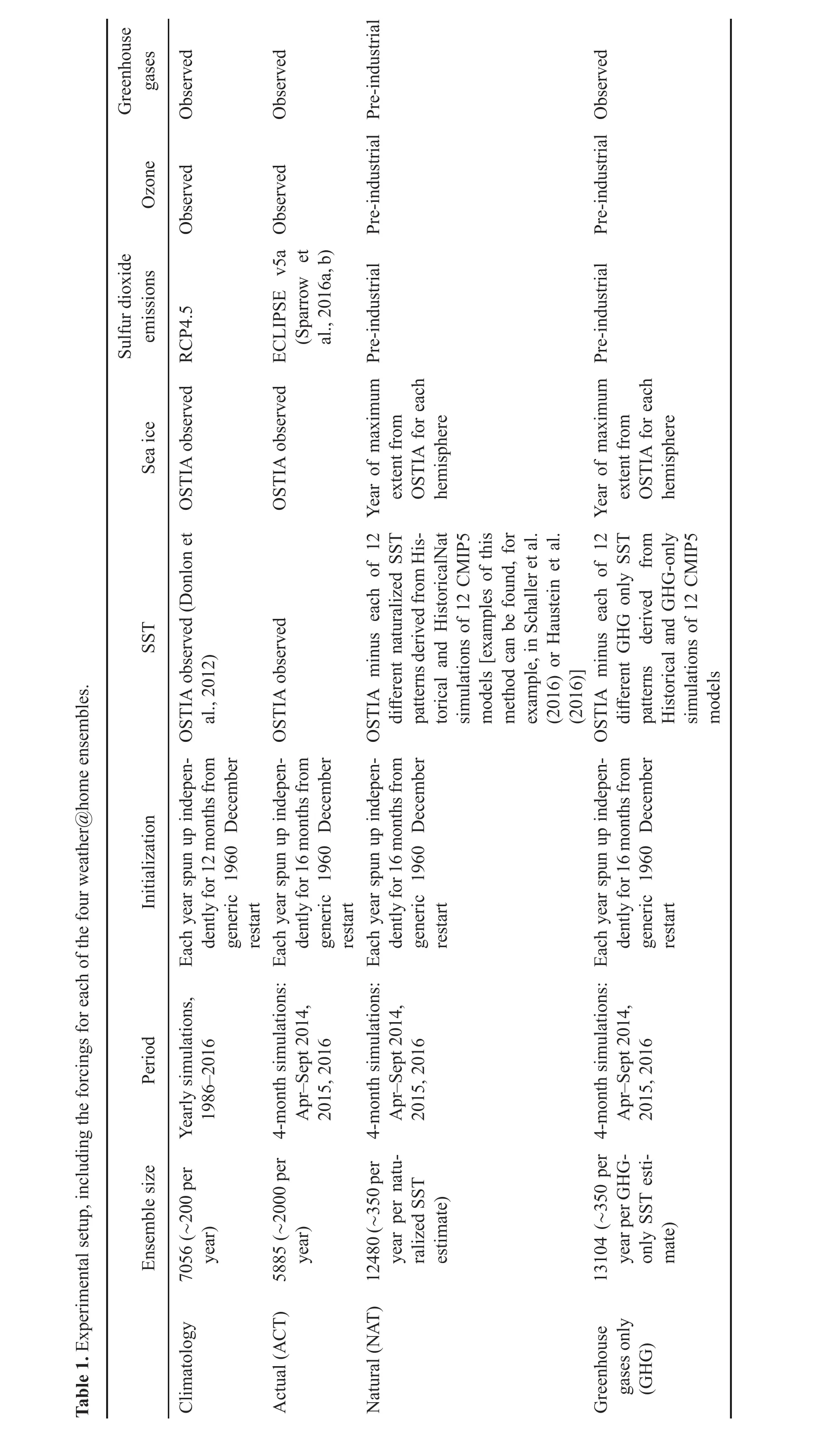
Four ensembles were conducted(Table 1):a 1986–2016 climatology,used for model evaluation(in which each year was run independently);and three repetitive single-year simulations forced by estimated natural forcings(NAT),greenhouse gases only(GHG),and observed aerosols and greenhouse gas emissions(ACT).These three simulations(NAT,GHG and ACT)repeated the same warm season(April–September)several thousand times with a small perturbation to the initial potential temperature field of the atmosphere.They were conducted for three different years(2014,2015 and 2016)and were each spun up for 16 months,i.e.,starting on 1 December two years prior to the study year.During this period,a strong El Niño event occurred,with a peak during the winter of 2015/16(Hu and Fedorov,2017).For this study,we consider summer 2014 as a reference(before the development of ENSO),summer 2015 as an ENSO year(with a strong signal even during the summer period),and 2016 as a following ENSO year or La-Niña-like year(Fig.1b).During 2016,the SST anomaly shows slightly warmer temperatures over the West Pacific and cooler SST over the central East Pacific(with magnitudes overall below 1◦C).Thus,2016 can also be considered as a weak negative ENSO phase,but these anomalies are relatively small compared to the 2015 patterns.

As the ACT ensemble corresponds most closely to reality,ACT-14(values of ACT in 2014)is used to compare against other years or cases.Thus,all results are presented as deviations compared to 2014.The difference between NAT and ACT represents the anthropogenic impact,while the difference between GHG and ACT gives an estimate of the impact of aerosols.

The model is evaluated by comparing the climatology of the highest daily maximum and minimum temperatures(TXx and TNx,respectively;Table 2)with results from ERA Interim(Dee et al.,2011),referred as ERAI in the figures.Although the simulated TXx values are too large compared to ERA-Interim over central and East China(Fig.S1),the spatial pattern is reproduced well.Comparing the model interannual variability and mean with ERA-Interim for Tmax and Tmin over central East China(Fig.S2),the model is warmer than ERA-Interim(especially Tmax)but cooler than the ground station observation.Moreover,it is consistent with the ERA-Interim trend and variability.The mean 2014–16 summer signal is also found to have a reasonable range compared to reanalysis and observation(Fig.S2),albeit the model mean is smoother due to ensemble averaging.The daily distribution of the temperatures over the region is also in good agreement with the observations(Fig.S3).The model performance is summarized with a Taylor diagram(Fig.S4)using ERA-Interim as a reference for all diagnostics.Spatial correlations are all above 0.9 and the variability of the model is close to ERA-Interim,albeit the most extreme temperatures(TXx and TNx)have slightly weaker scores than Tmax and Tmin.Station observations have weaker correlations with ERA-Interim than the model,which may be explained by their sparse spatial coverage compared to ERA Interim.

2.2.Index definition and computation

TX and TN are each used to compute several extreme indices during the extended summer(May–September):the summer maximum of each temperature(TXx and TNx,respectively,expressed in◦C)and the number of days above the 2014 climatological 95th percentile of each temperature(TX95 and TN95,expressed in days).Table 2 summarizes the notation and definitions.

The duration of the events is also considered,by selecting five-day persistent temperatures.To do so,the minimum temperature during the five-day time window is first selected(for each day of the summer),and then the maximum of these minima is extracted.For instance, first the minimum temperature is selected for 1–5 May,2–6 May...to 25–30 September.Then,the maximum among these minima is retained.

Each index is computed individually for each ensemble member before being analyzed as an ensemble.Thus,results are obtained for the GHG,NAT and ACT ensembles,and for 2014,2015 and 2016.

TXx and TNx are both fitted to generalized extreme value(GEV)distributions using,for each simulation,the maximum value at each grid point,in the extended summer season.Uncertainties in the parameter values are computed by bootstrapping(Efron and Tibshirani,1993)ACT-14 with 1000 samples and then computing the standard errors.The differences between ensembles are considered significant when they are larger than three standard deviations of the bootstrap ensemble(99.7%confidence interval).As there is a large number of members in each ensemble,the GEV fit is stable and uncertainties are small.

Most of the results are presented as differences between cases,and thus the systematic biases of the model are cancelled out.However,when presenting results as absolute temperatures,a bias correction is first applied.The model bias is estimated by simply computing the difference between the 2014 climatology and ERA-Interim(Fig.S1c and f),and removed from the model temperatures before being displayed in the figures.

3.Results

?

Fig.2.differences in the(a–h)location and(i–p)scale parameters from the GEV fit for each ensemble.All scales are in ◦C.Contours are every 0.2◦C and 0.05◦C intervals for the location and scale,respectively(with dashed lines indicating negative values).Only significant differences are shaded(see section 2 for details).

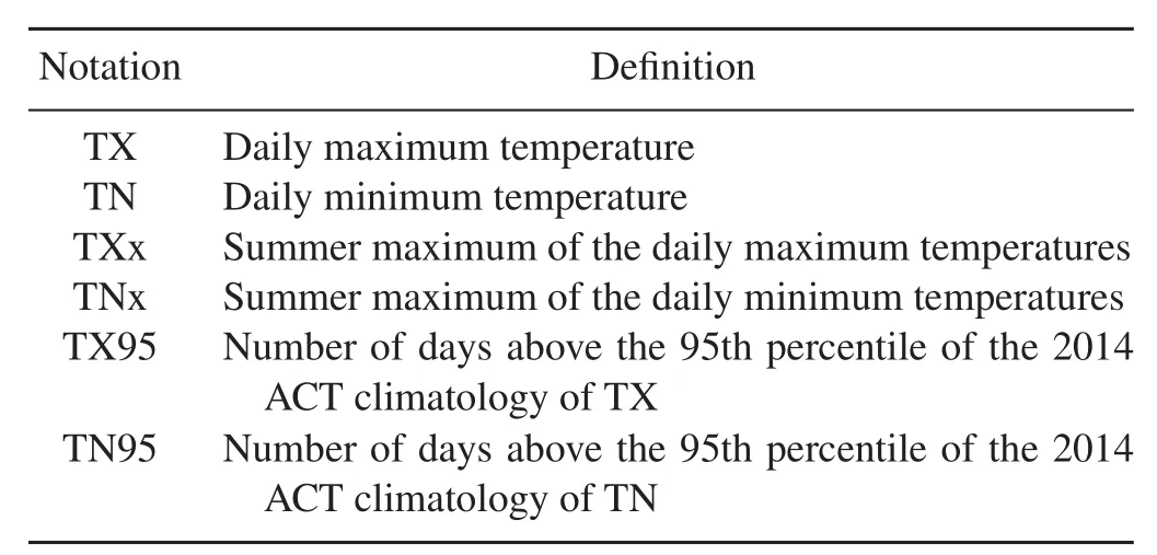
Table 2.Notation for the different types of indices.

The extended summer TXx and TNx are analyzed first.We use a GEV distribution to fit the ensemble distributions at each grid point and display the results in terms of location and scale parameters.Figure 2 displays the differences between each case,and the reference used for comparison(ACT-14)is also shown,in Fig.S5.The anthropogenic impact is quite clear and affects the temperatures over the whole region(Figs.2b and d)with an increase in the location parameter,and thus the mean summer TXx and TNx,of 1◦C to 1.5◦C.Conversely,aerosols tend to reduce the location parameter,by 0.5◦C to 1◦C(Figs.2a and c),consistent with previous findings(e.g.,Li et al.,2016).This suggests that well mixed greenhouse gases have increased the mean TXx and TNx.The scale parameter is found to be reduced by aerosols emissions(Figs.2i and k),by about 10%relative to the reference(Figs.S2c and d).This is especially the case for TNx,possibly due to the aerosols and their interaction with humidity.Another possibility is cooling reducing the potential land-surface amplification of extremes.However,this effect is small when considering all anthropogenic forcings(Figs.2j and l).This indicates that greenhouse gas emissions oppose the effect of aerosols and tend to increase the extreme temperature variability,leading to a small net effect.

The influence of ENSO(or more specifically,SST patterns)is more variable(Figs.2e–h).During the peak of the ENSO event(2015),extreme temperatures are reduced over central and Northeast China.This is especially so for TXx,for which the location parameter changes by 0.5◦C to 1◦C,which is of a similar magnitude to the impact of aerosols.

In the year after the event(2016),the impact is somewhat reversed,with an increase in temperatures over the eastern coastalregion(especially for TNx,with a magnitude of 0.5◦C to 1.2◦C).This is in accordance with Hu et al.(2013),who found an increase in hot days over the Yangtze River basin during El Niño years.This may be partly due to a warm SST anomaly(Fig.1c)in the Yellow Sea during 2015(Fig.1b).The reduction of TXx and TNx during the ENSO year is quite consistent with the negative anomaly of SST over the West Pacific(Fig.1b).Increased surface pressure over the West Pacific(Fig.S6)leads to cooler air being transported from the ocean to the continent and to milder temperatures over central China.Locally,the influence of ENSO or SST patterns can be considerable,potentially amplifying or off setting anthropogenic influences.The scale parameter mainly shows a reduction during and after ENSO,indicating less variability in extreme temperatures outside peak ENSO.This effect is local and does not correspond to the regions where the location parameter changes are the largest.

Similar results were analyzed for five-day persistent events(not shown).The patterns and magnitude of the differences were similar to the previous results,indicating that daily extremes and persistent extremes are impacted in the same way by the different drivers.

The shape parameter is also analyzed for daily extremes(Fig.S7).It does not show consistent large-scale signals;although,it can vary locally,indicating some changes in the tails of the distributions(i.e.,the most extreme values).Most of the differences,however,are not significant.

As a complement to the most extreme temperatures,we also analyze the probability of temperatures exceeding their respective climatological 95th percentiles(Fig.S8).Similar to TXx and TNx,the anthropogenic influence is quite homogenous and increases TX95 and TN95 by 30%to 60%compared to the naturalized case(Fig.S8b and d).Aerosols produce stronger and more variable spatial patterns(Figs.S8a and c)than greenhouse gases,especially for TN95.Along the coastal regions,TN95 is more than doubled in GHG compared to ACT.Thus,aerosols halve the probability of nighttime high temperatures over these regions.This pattern is not visible for TX95,and as these coastal regions have overall more humidity than central regions it indicates again that aerosols have strong interaction with humidity(and thus nighttime temperatures).This may be an indirect effect of aerosols insofar as they tend to cool down the SST and thus lower the overall atmospheric humidity,especially over coastal regions.

The impact of ENSO on TX95 and TN95(Figs.S8e–h)is similar to TXx and TNx.During 2015,TX95 and TN95 are both reduced by more than 40%over central China;whereas,after the ENSO event,TN95 is approximately doubled over the eastern coast.Thus,ENSO has a more consistent impact on the temperatures:it tends to reduce(during)or enhance(after)both the high(above the 95th percentile)and maximum temperatures,while the aerosols lead to a variable response.

To summarize the impact of ENSO over the central China region(orange box in Fig.1a),the distribution of the regional-averaged TXx and TNx is computed and displayed(Fig.3)in terms of estimated return periods.TXx and TNx are bias-corrected first(see section 2).During the ENSO year,the return times of TXx are strongly reduced,so extreme high temperatures become less probable.For instance,a 1-in-10-year return event becomes a 1-in-50-year return event during 2015.This shift is similar for all return periods(although,it follows a logarithmic scale,meaning the effect on the highest return periods is amplified).Each case(ACT,GHG and NAT)shows the same signal,albeit it is stronger in ACT.This may be because ACT uses observed SSTs,while the other cases use modified SSTs to be consistent with the emissions or naturalized world scenario(thus,the actual pattern of ENSO may be altered).The signal is weaker for TNx,although it is still visible for each case.The anthropogenic and aerosol impacts are also quite clear,with a large shift be-tween the di ff erent cases.

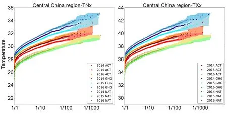
Fig.3.Return period of central China(25◦–35◦N,110◦–117E)regional-mean temperatures(units: ◦C)for each ensemble and year(colored circles)and their respective 95%confidence interval(shading).The temperatures are first bias-corrected,by removing the corresponding regional mean differences(based on the 2014 climatology)between HadRM3P and ERA-Interim(Figs.S1c and f).

The same investigation is conducted for coastal East China(Fig.S9,and Fig.1a for the definition of the region).TNx is the most impacted over this region during the post-ENSO year,and the signal is clearly visible for all cases and all return periods.TXx does not exhibit a clear shift during the post-ENSO year,but the shift during 2015 is visible.Thus,the ENSO impact on TXx is not limited to the central China region(although it is clearer there).

Finally,to complete the statistical approach of the study,the differences in the atmospheric circulation between each case are investigated(Fig.S6).In Had RM3P,the main differences are found for sea level pressure(SLP).During 2015,a positive anomaly extends over the West Pacific to the South Asia region.This leads to enhanced air transport from the ocean to the continent and thus moderates the temperature over central China(lower TXx).During 2016,a positive SLP anomaly is also visible over the West Pacific but it does not extend over the continent.This may lead to enhanced circulation near the coast(with possibly higher humidity and thus enhanced TNx),while central China temperatures remain more impacted by land–atmosphere processes(thus,higher TXx).The differences between the Had RM3P ensembles(ACT minus GHG and ACT minus NAT)are much weaker and suggest that the anthropogenic impact on temperature is mainly due to thermodynamic effects.It is also noticeable that the anomalies in ERA-Interim are different from the model,especially in the mid-upper troposphere.This may be due to the ensemble averaging,where only the most systematic anomalies remain.

Finally,the seasonal signal of TX and TN is analyzed by extracting the day corresponding to TXx and TNx in each member(ensemble results displayed in Fig.4 for the differences,and Figs.S5g and h for the reference).The results show that when we consider all anthropogenic forcings,or the forcing of aerosols alone,the effect on the timing of the maxima is only slight(Figs.4a–d).ENSO exhibits a dipole pattern during the event(Figs.4e and g),with the hottest day occurring earlier in South China and later in North China,and an overall delay after the event(Figs.4f and h).As we only consider one ENSO event,it does not mean that the seasonality of the extreme temperatures is systematically modified in the same way(during and just after the event),but mainly that changes in SST patterns modify the seasonal timing of extreme temperatures.

4.Conclusion

The influence of anthropogenic forcings(mainly greenhouse gases and aerosols)and natural variability(using the 2015/16 ENSO event)on summer extreme temperatures over China is analyzed with multi-thousand-member ensembles.This method allows a strong statistical analysis for a single ENSO event and for the most extreme temperatures in an extended summer,albeit the results are only based on results from a single model.

During the peak of ENSO,TXx is reduced significantly over the central China region.In 2016(post ENSO)TNx tends to increase over the eastern coastal region.The magnitude of the year-to-year anomalies is as large as the anthropogenic influence.This implies that the natural variability can influence,at a regional scale,in a significant way,extreme temperatures.Based on the model,ENSO can oppose,during the peak of the event,or amplify,the following year,the effect of greenhouse gases on summer temperature extremes.The overall return-period probability is also found to be reduced for both TX and TN during El Niño.The impact is mainly observed on the location parameters of the GEV fitting,meaning it is mainly due to a shift in temperatures rather than a change in variability.

Aerosols have a strong signature in TNx over the coastal region,perhaps indicating an effect of aerosols on the humidity(including reduced evaporation due to the cooling effect,or potential changes in cloud properties).Although this is an interesting point,more experiments are needed for a better understanding.

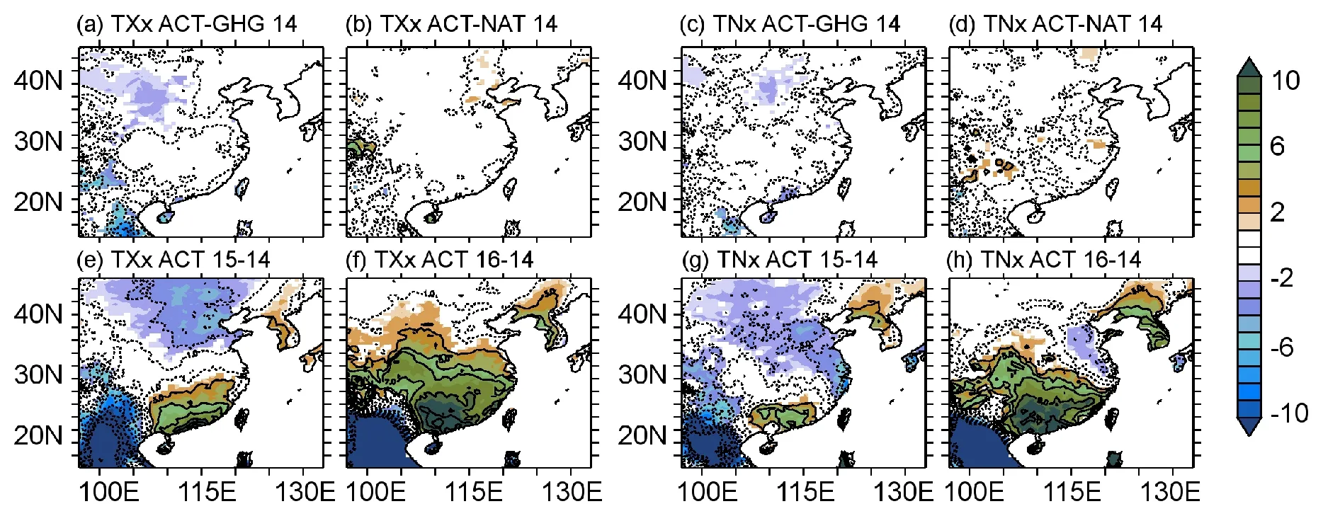
Fig.4.difference in the ensemble means of the average time of TXx and TNx in days.Contours are in two-day intervals(with dashed lines indicating negative values).Positive(negative)values correspond to a delay(advance)in the peak of temperatures.Shaded values are above the 99.7%confidence interval.

Finally,the timing of the maximum temperatures during the summer shifts by more than 10 days between the year 2016 and 2014(whereas,the anthropogenic forcings did not impact this shift).This highlights how ENSO can quickly modify the seasonality of extreme temperatures,and should be an important point for seasonal forecasting.

This study indicates that,based on model results,natural interannual variability and anthropogenic forcing have similar magnitudes of impact on extreme temperatures over China.Although,the former has a more regional effect,while the latter has a more spatially homogenous signal.

It should be noted that this study considers only one specific ENSO event,which had a strong signal during the summer.Other ENSO events could have different impacts,depending on their SST patterns and timing.Moreover,given the possible biases in the model,the magnitude of the response in the real world could be different.We are highly confident that the patterns are realistic,given that the model has very good skill in reproducing TXx and TNx spatial characteristics.

Acknowledgements.This work and all contributors were supported by the UK–China Research and Innovation Partnership Fund through the Met Office Climate Science for Service Partnership(CSSP)China as part of the Newton Fund.We would like to thank the Met Office Hadley Centre PRECIS team for their technical and scientific support for the development and application of weather@home.Finally,we would like to thank all of the volunteers who have donated their computing time to climate prediction.net and weather@home.

Open AccessThis article is distributed under the terms of the Creative Commons Attribution License which permits any use,distribution,and reproduction in any medium,provided the original author(s)and the source are credited.

Electronic supplementary material:Supplementary material is available in the online version of this article at https://doi.org/10.1007/s00376-018-7258-8.

REFERENCES

Black,M.T.,and D.J.Karoly,2016:Southern Australia’swarmest October on record:The role of ENSO and climate change.Bull.Amer.Meteor.Soc.,97,S118–S121,https://doi.org/10.1175/BAMS-D-16-0124.1.

Black,M.T.,and Coauthors,2016:The weather@home regional climate modelling project for Australia and New Zealand.Geoscientific Model Development,9,3161–3176,https://doi.org/10.5194/gmd-9-3161-2016.

Chen,Y.,and P.M.Zhai,2017:Revisiting summertime hot extremes in China during 1961-2015:Overlooked compound extremes and significant changes.Geophys.Res.Lett.,44,5096–5103,https://doi.org/10.1002/2016GL072281.

Dee,D.P.,and Coauthors,2011:The ERA-Interim reanalysis:Configuration and performance of the data assimilation system.Quart.J.Roy.Meteor.Soc.,137(656),553–597,https://doi.org/10.1002/qj.828.

Dong,B.W.,R.T.Sutton,and L.Shaffrey,2017:Understanding the rapid summer warming and changes in temperature extremes since the mid-1990s over Western Europe.Climate Dyn.,48,1537–1554,https://doi.org/10.1007/s00382-016-3158-8.

Donlon,C.J.,M.Martin,J.Stark,J.Roberts-Jones,E.Fiedler,and W.Wimmer,2012:The Operational Sea Surface Temperature and Sea Ice analysis(OSTIA)system.Remote Sensing of Environment,116,140–158,https://doi.org/10.1016/j.rse.2010.10.017.

Efron,B.,and R.J.Tibshirani,1993:An Introduction to the Bootstrap.Chapman and Hall.

Essery,R.and D.B.Clark,2003:Developments in the MOSES 2 land-surface model for PILPS 2e.Global Planet Change,38,161–164,https://doi.org/10.1016/S0921-8181(03)00026-2.

Freychet,N.,S.Tett,J.Wang,and G.Hegerl,2017:Summer heat waves over Eastern China:Dynamical processes and trend attribution.Environmental Research Letters,12,024015,https://doi.org/10.1088/1748-9326/aa5ba3.

Guillod,B.P.,and Coauthors,2017:weather@home 2:validation of an improved global-regional climate modelling system.Geosci.Model Dev.,10,1849–1872,https://doi.org/10.5194/gmd-10-1849-2017.

Haustein,K.,and Coauthors,2016:Real-time extreme weather event attribution with forecast seasonal SSTs.Environmental Research Letters,11,064006,https://doi.org/10.1088/1748-9326/11/6/064006.

Hu,K.M.,G.Huang,and R.G.Wu,2013:A strengthened influence of ENSO on August high temperature extremes over the Southern Yangtze River Valley since the Late 1980s.J.Climate,26,2205–2221,https://doi.org/10.1175/JCLI-D-12-00277.1.

Hu,S.N.,and A.V.Fedorov,2017:The extreme El Niño of 2015–2016 and the end of global warming hiatus.Geophys.Res.Lett.,44,3816–3824,https://doi.org/10.1002/2017 GL072908.

Jones,A.,D.L.Roberts,M.J.Woodage,&C.E.Johnson,2001:Indirect sulphate aerosol forcing in a climate model with an interactive sulphur cycle.J.Geophys.Res.:Atmospheres,106(D17),20293–20310,https://doi.org/10.1029/2000JD000089.

Kasoar,M.,A.Voulgarakis,J.-F.Lamarque,D.T.Shindell,N.Bellouin,W.J.Collins,G.Faluvegi,and K.Tsigaridis,2016:Regional and global temperature response to anthropogenic SO2emissions from China in three climate models.Atmospheric Chemistry and Physics,16,9785–9804,https://doi.org/10.5194/acp-16-9785-2016.

Li,C.X.,T.B.Zhao,and K.R.Ying,2016:Effects of anthropogenic aerosols on temperature changes in China during the twentieth century based on CMIP5 models.Theor.Appl.Climatol.,125,529–540,https://doi.org/10.1007/s00704-015-1527-6.

Li,S.H.,P.W.Mote,D.E.Rupp,D.Vickers,R.Mera,and M.Allen,2015:Evaluation of a regional climate modeling effort for the Western United States using a superensemble from weather@home.J.Climate,28,7470–7488,https://doi.org/10.1175/JCLI-D-14-00808.1.

Luo,M.,and N.-G.Lau,2017:Heat waves in Southern China:Synoptic behavior,long-term change,and urbanization effects.J.Climate,30(2),703–720,https://doi.org/10.1175/JCLI-D-16-0269.1.

Ma,S.M.,T.J.Zhou,D.A.Stone,O.Ang´elil,and H.Shiogama,2017:Attribution ofthe July–August2013 heatevent in Central and Eastern China to anthropogenic greenhouse gas emissions.Environmental Research Letters,12,054020,https://doi.org/10.1088/1748-9326/aa69d2.

Marthews,T.R.,F.E.L.Otto,D.Mitchell,S.J.Dadson,and R.G.Jones,2015:The 2014 drought in the Horn of Africa:Attribution of meteorological drivers.Bull.Amer.Meteor.Soc.,96,S83–S88,https://doi.org/10.1175/BAMS-D-15-00115.1.

Mascioli,N.R.,A.M.Fiore,M.Previdi,and G.Correa,2016:Temperature and precipitation extremes in the United States:Quantifying the responses to anthropogenic aerosols and greenhouse gases.J.Climate,29,2689–2701,https://doi.org/10.1175/JCLI-D-15-0478.1.

McPhaden,M.J.,S.E.Zebiak,and M.H.Glantz,2016:ENSO as an integrating concept in earth science.Science,314,1740–1745,https://doi.org/10.1126/science.1132588.

Mitchell,D.,and Coauthors,2016:Attributing human mortality during extreme heat waves to anthropogenic climate change.Environmental Research Letters,11,074006,https://doi.org/10.1088/1748-9326/11/7/074006.

Otto,F.E.L.,2017:Attribution of weather and climate events.Annual Review of Environment and Resources,42,627–646,https://doi.org/10.1146/annurev-environ-102016-060847.

Peng,X.,Q.N.She,L.B.Long,M.Liu,Q.Xu,J.X.Zhang,and W.N.Xiang,2017:Long-term trend in ground-based air temperature and its responses to atmospheric circulation and anthropogenic activity in the Yangtze River Delta,China.Atmospheric Research,195,20–30,https://doi.org/10.1016/j.atmosres.2017.05.013.

Qian,C.,and Coauthors,2018:Human in fluence on the record breaking cold event in January of 2016 in Eastern China.Bull.Amer.Meteor.Soc.,99(1),S118–S122,https://doi.org/10.1175/BAMS-D-17-0095.1.

Ren,Y.-Y.,D.Parker,G.-Y.Ren,and R.Dunn,2016:Tempospatial characteristics of sub-daily temperature trends in mainland China.Climate Dyn.,46,2737–2748,https://doi.org/10.1007/s00382-015-2726-7.

Sarofim,M.C.,and Coauthors,2016:Temperature-related death and illness.Chapter 2,The Impacts of Climate Change onHuman Health in the United States:A Scientific Assessment,U.S.Global Change Research Program,43–68.

Sarojini,B.B.,P.A.Stott,and E.Black,2016:Detection and attribution of human influence on regional precipitation.Nature Climate Change,6(7),669–675,https://doi.org/10.1038/nclimate2976.

Schaller,N.,and Coauthors,2016:Human in fluence on climate in the 2014 southern England winter floods and their impacts.Nature Climate Change,6,627–634,https://doi.org/10.1038/nclimate2927.

Sparrow,S.,D.Wallom,Z.Klimont,C.Hayes,and W.Ingram,2016a:1990 to 2050 Atmospheric SO2Ancillary Files for HadCM3.[Available online from https://figshare.com/articles/Atmospheric_SO2_Ancillary_Files_for_HadCM3/3409186]

Sparrow,S.,D.Wallom,and W.Ingram,2016b:Sulphate Ancillary Metadata and Processing Metadata and Scripts. figshare.https://doi.org/10.6084/m9.figshare.3469199.v3.

Sun,Q.H.,C.Y.Miao,A.AghaKouchak,and Q.Y.Duan,2017:Unraveling anthropogenic influence on the changing risk of heat waves in China.Geophys.Res.Lett.,44,5078–5085,https://doi.org/10.1002/2017GL073531.

Sun,Y.,L.C.Song,H.Yin,B.T.Zhou,T.Hu,X.B.Zhang and P.Stott,2016:Human influence on the 2015 extreme high temperature events in Western China.Bull.Amer.Meteor.Soc.,97(12),S102–S106,https://doi.org/10.1175/BAMS-D-16-0158.1.

Yin,H.,Y.Sun,H.Wan,X.B.Zhang,and C.H.Lu,2017:Detection of anthropogenic influence on the intensity of extreme temperaturesin China.Int.J.Climatol.,37,1229–1237,https://doi.org/10.1002/joc.4771.

Zhang,H.H.,T.L.Delworth,F.R.Zeng,G.Vecchi,K.Paffendorf,and L.W.Jia,2016:Detection,attribution,and projection of regional rainfall changes on(multi-)decadal time scales:A focus on Southeastern South America.J.Climate,29,8515–8534,https://doi.org/10.1175/JCLI-D-16-0287.1.

Zhou,C.-L.,and K.-C.Wang,2016:Coldest temperature extreme monotonically increased and hottest extreme oscillated over Northern hemisphere land during last 114 years.Scientific Reports,6,25721,https://doi.org/10.1038/srep25721.